探索的解析と品質管理
Last updated on 2026-04-28 | Edit this page
Estimated time 180 minutes
Overview
Questions
- RNA-seq解析において、探索的解析がなぜ重要なステップなのでしょうか?
- 探索的解析を行う際、生のカウント行列をどのように前処理すべきですか?
- データを表現するために2次元で十分なのでしょうか?
Objectives
- 遺伝子発現マトリックスの解析方法と、一般的な品質管理手順を習得します。
- 探索的解析用のインタラクティブなアプリケーション環境の構築方法を学びます。
パッケージの読み込み
RStudioを再起動した直後の状態を想定して、このレッスンで使用するパッケージと、前回のレッスンで作成した
SummarizedExperiment オブジェクトを読み込みます。
R
suppressPackageStartupMessages({
    library(SummarizedExperiment)
    library(DESeq2)
    library(vsn)
    library(ggplot2)
    library(ComplexHeatmap)
    library(RColorBrewer)
    library(hexbin)
    library(iSEE)
})
R
se <- readRDS("data/GSE96870_se.rds")
発現していない遺伝子の除去
探索的解析は、データの品質管理と理解において非常に重要なプロセスです。 これにより、データ品質の問題、サンプルの取り違え、コンタミネーションなどを検出できるほか、データ中に存在する顕著なパターンを把握することも可能になります。 本エピソードでは、RNA-seqデータに対する探索的解析の代表的な手法であるクラスタリングと主成分分析(PCA)の2つについて解説します。 これらのツールはRNA-seqデータの解析に限定されたものではなく、他の種類のデータ解析にも応用可能です。 ただし、カウントベースのアッセイにはこの種のデータに適用する際に考慮すべき特有の特徴があります。まず第一に、ゲノム上のすべてのマウス遺伝子が小脳サンプルで発現しているわけではありません。遺伝子の発現が検出可能かどうかを判断するための閾値は複数存在しますが、ここでは非常に厳格な基準を採用します。具体的には、全サンプルを通じて遺伝子の総カウント数が5未満の場合、そもそもデータ量が不足しており、有効な解析を行うことができないものとします。
R
nrow(se)
OUTPUT
[1] 41786R
# Remove genes/rows that do not have > 5 total counts
se <- se[rowSums(assay(se, "counts")) > 5, ]
nrow(se)
OUTPUT
[1] 27430課題:このフィルタリングを通過した遺伝子にはどのような特徴があるのか?
前回のエピソードでは、mRNA遺伝子のみに絞り込むサブセット処理について議論しました。今回はさらに、最低限の発現レベルを基準にサブセット処理を行いました。
- 各種類の遺伝子のうち、フィルタリングを通過した遺伝子の数はそれぞれどれくらいでしょうか?
- 異なる閾値を用いてフィルタリングを通過した遺伝子数を比較してください。
- より厳格なフィルタリングを行う場合の利点と欠点は何でしょうか?また、考慮すべき重要な点にはどのようなものがあるでしょうか?
R
table(rowData(se)$gbkey)
OUTPUT
     C_region          exon     J_segment      misc_RNA          mRNA
           14          1765            14          1539         16859
        ncRNA precursor_RNA          rRNA          tRNA     V_segment
         6789           362             2            64            22
R
nrow(se) # represents the number of genes using 5 as filtering threshold
OUTPUT
[1] 27430R
length(which(rowSums(assay(se, "counts")) > 10))
OUTPUT
[1] 25736R
length(which(rowSums(assay(se, "counts")) > 20))
OUTPUT
[1] 23860- Cons: 興味深い情報を削除するリスク Pros:
- 発現量が低いまたは検出限界以下の遺伝子は、生物学的に有意な結果をもたらす可能性が低いと考えられます。
- 統計的検定の回数を削減できます(多重検定の問題を軽減)。
- 平均値と分散の関係をより信頼性の高い方法で推定できます。
考慮すべき事項: - 両群において当該遺伝子は発現していますか? - 各群で当該遺伝子を発現しているサンプル数はいくつですか?
ライブラリサイズの差異について
サンプル間で遺伝子に割り当てられた総リード数に差異が生じる場合、これは主に技術的な要因によるものです。実際には、単に遺伝子の生のリードカウントをサンプル間で直接比較し、リード数が多いサンプルほどその遺伝子の発現量が多いと結論づけることはできません。高いリードカウントは、そのサンプルにおける総リード数が全体的に多いことに起因している可能性があるためです。 本節の残りの部分では、「ライブラリサイズ」という用語を、サンプルごとに遺伝子に割り当てられた総リード数を指すものとして使用します。まずすべてのサンプルのライブラリサイズを比較する必要があります。
R
# Add in the sum of all counts

se$libSize <-  colSums(assay(se))

# Plot the libSize by using R's native pipe |>
# to extract the colData, turn it into a regular
# data frame then send to ggplot:

colData(se) |>
  as.data.frame() |>
  ggplot(aes(x = Label, y = libSize / 1e6, fill = Group)) +
         geom_bar(stat = "identity") + theme_bw() +
         labs(x = "Sample", y = "Total count in millions") +
         theme(axis.text.x = element_text(angle = 45, hjust = 1, vjust = 1))
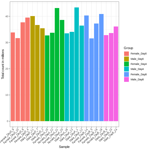
サンプル間のライブラリサイズの差異を適切に補正しなければ、誤った結論を導く危険性があります。RNA-seqデータにおいてこの処理を行う標準的な方法は、2段階の手順で説明できます。 まず、サンプルごとに固有の補正係数である「サイズ因子」を推定します。これらの因子を用いて生のカウント値を除算すれば、サンプル間でより比較可能な値が得られるようになります。 次に、これらのサイズ因子をデータの統計解析プロセスに組み込みます。 重要なのは、特定の解析手法においてこの処理がどのように実装されているかを詳細に確認することです。 場合によっては、アナリスト自身がカウント値をサイズ因子で明示的に除算する必要があることもあります。 また別のケースでは(差異発現解析で後述するように)、これらを解析ツールに別途提供することが重要です。ツールはこれらの因子を適切に統計モデルに適用します。
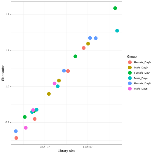
DESeq2では、estimateSizeFactors()関数を用いてサイズ因子を計算します。
この関数で推定されるサイズ因子は、ライブラリサイズの差異補正と、サンプル間のRNA組成の差異補正を組み合わせたものです。
後者は特に重要です。RNA-seqデータは組成的な性質を持つため、遺伝子間で分配されるリード数には一定の上限があります。もし特定の遺伝子(あるいは少数の非常に高発現遺伝子)がリードの大部分を占有すると、他のすべての遺伝子は必然的に非常に低いカウント値しか得られなくなります。ここで私たちは、内部構造としてこれらのサイズ因子を格納できるDESeqDataSetオブジェクトにSummarizedExperimentオブジェクトを変換します。また、主要な実験デザイン(性別と時間)を指定する必要もあります。
R
dds <- DESeq2::DESeqDataSet(se, design = ~ sex + time)
WARNING
Warning in DESeq2::DESeqDataSet(se, design = ~sex + time): some variables in
design formula are characters, converting to factors
R
dds <- estimateSizeFactors(dds)

# Plot the size factors against library size
# and look for any patterns by group:

ggplot(data.frame(libSize = colSums(assay(dds)),
                  sizeFactor = sizeFactors(dds),
                  Group = dds$Group),
       aes(x = libSize, y = sizeFactor, col = Group)) +
    geom_point(size = 5) + theme_bw() +
    labs(x = "Library size", y = "Size factor")
データの前処理
探索的解析のための手法に関する研究文献は数多く存在します。 これらの手法の多くは、入力データ(ここでは各遺伝子)の分散が平均値から比較的独立している場合に最も効果的に機能します。 RNA-seqのようなリードカウントデータの場合、この前提は成立しません。 実際には、分散は平均リードカウントの増加に伴って増大する傾向があります。
R
meanSdPlot(assay(dds), ranks = FALSE)
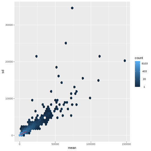
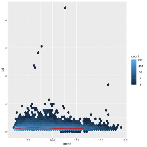
この問題に対処する方法は2つあります:1つ目は、カウントデータに特化した分析手法を開発する方法、2つ目は既存の手法を適用できるようにカウントデータを変換する方法です。 どちらの方法も研究されてきましたが、現時点では後者のアプローチの方が実際に広く採用されています。具体的には、DESeq2の分散安定化変換を用いてデータを変換した後、平均リードカウントと分散の相関関係が適切に除去されていることを確認できます。
R
vsd <- DESeq2::vst(dds, blind = TRUE)
meanSdPlot(assay(vsd), ranks = FALSE)
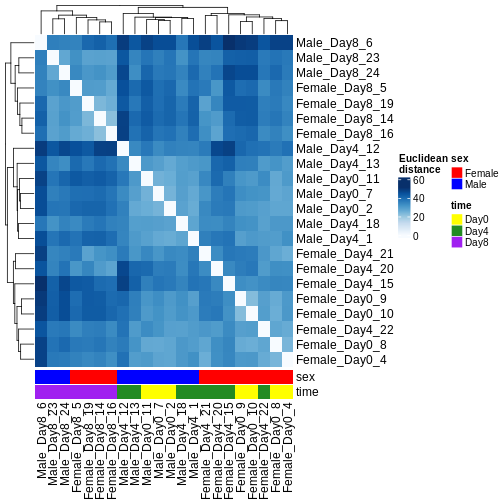
ヒートマップとクラスタリング解析
発現パターンの類似性に基づいてサンプルをクラスタリングする方法は複数存在します。最も単純な手法の一つは、すべてのサンプルペア間のユークリッド距離を計算することです(距離が長いほど類似性が低いことを示します)。その後、分岐型デンドログラムとヒートマップの両方を用いて結果を可視化し、距離を色で表現します。この解析から、Day 8のサンプルは他のサンプル群と比較して互いにより類似していることが明らかになりました。ただし、Day 4とDay 0のサンプルは明確には分離していません。代わりに、雄個体と雌個体は確実に分離することが確認されました。
R
dst <- dist(t(assay(vsd)))
colors <- colorRampPalette(brewer.pal(9, "Blues"))(255)
ComplexHeatmap::Heatmap(
    as.matrix(dst),
    col = colors,
    name = "Euclidean\ndistance",
    cluster_rows = hclust(dst),
    cluster_columns = hclust(dst),
    bottom_annotation = columnAnnotation(
        sex = vsd$sex,
        time = vsd$time,
        col = list(sex = c(Female = "red", Male = "blue"),
                   time = c(Day0 = "yellow", Day4 = "forestgreen", Day8 = "purple")))
)
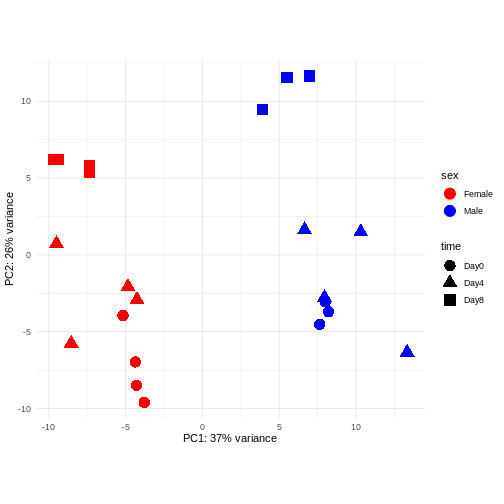
主成分分析(PCA)
主成分分析は次元削減手法の一つであり、サンプルデータを低次元空間に投影する手法である。 この低次元表現は、データの可視化や、さらなる分析手法の入力データとして利用することができる。 主成分は、互いに直交するように定義され、それらが張る空間へのサンプル投影が可能な限り多くの分散情報を保持するように設計されている。 この手法は教師なし学習の一種であり、サンプルに関する外部情報(例えば処理条件など)は一切考慮されない。 以下の図では、サンプルを2次元の主成分空間に投影して表現している。 各次元について、当該成分が説明する全分散の割合を示している。 定義上、第1主成分は常に後続する主成分よりも多くの分散を説明することになる。 説明分散率とは、元の高次元空間から低次元空間にデータを投影して可視化する際に、データ中の「信号」成分のうちどの程度が保持されているかを示す指標である。
R
pcaData <- DESeq2::plotPCA(vsd, intgroup = c("sex", "time"),
                           returnData = TRUE)
OUTPUT
using ntop=500 top features by varianceR
percentVar <- round(100 * attr(pcaData, "percentVar"))
ggplot(pcaData, aes(x = PC1, y = PC2)) +
    geom_point(aes(color = sex, shape = time), size = 5) +
    theme_minimal() +
    xlab(paste0("PC1: ", percentVar[1], "% variance")) +
    ylab(paste0("PC2: ", percentVar[2], "% variance")) +
    coord_fixed() +
    scale_color_manual(values = c(Male = "blue", Female = "red"))
課題:隣の人と以下の点について話し合ってください
主に感染後の時間経過に伴う発現変化(Reminder Day0時点 -> 感染前)に関心がある場合、下流解析で考慮すべき点は何でしょうか?
同一ドナーから複数のサンプルを取得した実験デザインを考えてみましょう。あなたは引き続き時間差による差異に関心があり、以下のPCAプロットを観察しました。このPCAプロットからどのような示唆が得られるでしょうか?
OUTPUT
using ntop=500 top features by variance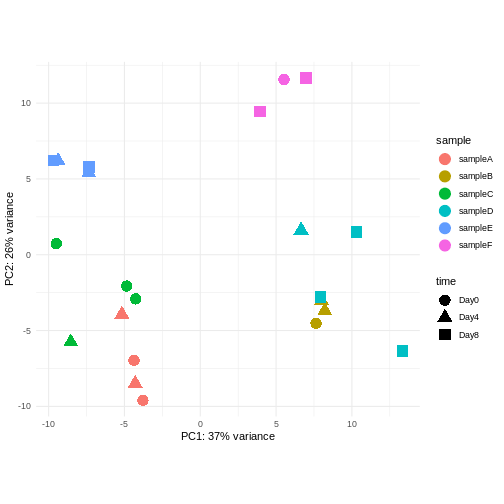
このデータにおける主要なシグナル(分散の37%)は性別と関連しています。私たちは時間経過に伴う性特異的な変化には関心がないため、下流解析ではこの影響を調整する必要があります(次のエピソード参照)。また、今後の探索的下流解析においてもこの要因を考慮に入れておく必要があります。この影響を補正する方法として、性染色体上に位置する遺伝子を除去することが考えられます。
- 考慮すべき強いドナー効果が認められます。
- PC1(分散の37%)は何を表しているのでしょうか? これは2つのドナーグループを示しているように思われます。
- PC1とPC2には時間との関連性が認められません → 時間による転写レベルの影響は存在しないか、あるいは弱いと考えられます --> より高次の主成分(例:PC3、PC4、…)との関連性を確認してください
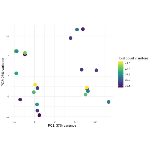
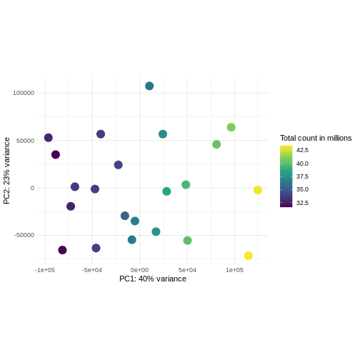
課題: ライブラリサイズに応じて色分けしたPCAプロットを作成してください
分散安定化変換前後の結果を比較してください。
ヒント:
DESeq2::plotPCA関数は入力としてDESeqTransformクラスのオブジェクトを期待します。SummarizedExperimentオブジェクトを変換するには、plotPCA(DESeqTransform(se))と記述します
R
pcaDataVst <- DESeq2::plotPCA(vsd, intgroup = c("libSize"),
                              returnData = TRUE)
OUTPUT
using ntop=500 top features by varianceR
percentVar <- round(100 * attr(pcaDataVst, "percentVar"))
ggplot(pcaDataVst, aes(x = PC1, y = PC2)) +
    geom_point(aes(color = libSize / 1e6), size = 5) +
    theme_minimal() +
    xlab(paste0("PC1: ", percentVar[1], "% variance")) +
    ylab(paste0("PC2: ", percentVar[2], "% variance")) +
    coord_fixed() +
    scale_color_continuous("Total count in millions", type = "viridis")
R
pcaDataCts <- DESeq2::plotPCA(DESeqTransform(se), intgroup = c("libSize"),
                              returnData = TRUE)
OUTPUT
using ntop=500 top features by varianceR
percentVar <- round(100 * attr(pcaDataCts, "percentVar"))
ggplot(pcaDataCts, aes(x = PC1, y = PC2)) +
    geom_point(aes(color = libSize / 1e6), size = 5) +
    theme_minimal() +
    xlab(paste0("PC1: ", percentVar[1], "% variance")) +
    ylab(paste0("PC2: ", percentVar[2], "% variance")) +
    coord_fixed() +
    scale_color_continuous("Total count in millions", type = "viridis")
インタラクティブな探索的データ解析
実験要因を詳細に調査したり、コーディング経験のない関係者から知見を得たりする場合、QCプロットをインタラクティブに操作しながら分析することが非常に有効です。RNA-seqデータの探索的データ分析に有用なツールとして、GlimmaとiSEEが挙げられます。
Challenge: Interactively explore our data using iSEE
R
## Convert DESeqDataSet object to a SingleCellExperiment object, in order to
## be able to store the PCA representation
sce <- as(dds, "SingleCellExperiment")

## Add PCA to the 'reducedDim' slot
stopifnot(rownames(pcaData) == colnames(sce))
reducedDim(sce, "PCA") <- as.matrix(pcaData[, c("PC1", "PC2")])

## Add variance-stabilized data as a new assay
stopifnot(colnames(vsd) == colnames(sce))
assay(sce, "vsd") <- assay(vsd)

app <- iSEE(sce)
shiny::runApp(app)
Session info
R
sessionInfo()
OUTPUT
R version 4.5.3 (2026-03-11)
Platform: x86_64-pc-linux-gnu
Running under: Ubuntu 22.04.5 LTS

Matrix products: default
BLAS:   /usr/lib/x86_64-linux-gnu/blas/libblas.so.3.10.0
LAPACK: /usr/lib/x86_64-linux-gnu/lapack/liblapack.so.3.10.0  LAPACK version 3.10.0

locale:
 [1] LC_CTYPE=C.UTF-8       LC_NUMERIC=C           LC_TIME=C.UTF-8
 [4] LC_COLLATE=C.UTF-8     LC_MONETARY=C.UTF-8    LC_MESSAGES=C.UTF-8
 [7] LC_PAPER=C.UTF-8       LC_NAME=C              LC_ADDRESS=C
[10] LC_TELEPHONE=C         LC_MEASUREMENT=C.UTF-8 LC_IDENTIFICATION=C

time zone: UTC
tzcode source: system (glibc)

attached base packages:
[1] grid      stats4    stats     graphics  grDevices utils     datasets
[8] methods   base

other attached packages:
 [1] iSEE_2.20.0                 SingleCellExperiment_1.30.1
 [3] hexbin_1.28.5               RColorBrewer_1.1-3
 [5] ComplexHeatmap_2.24.1       ggplot2_3.5.2
 [7] vsn_3.76.0                  DESeq2_1.48.1
 [9] SummarizedExperiment_1.38.1 Biobase_2.68.0
[11] MatrixGenerics_1.20.0       matrixStats_1.5.0
[13] GenomicRanges_1.60.0        GenomeInfoDb_1.44.0
[15] IRanges_2.42.0              S4Vectors_0.46.0
[17] BiocGenerics_0.54.0         generics_0.1.4

loaded via a namespace (and not attached):
 [1] rlang_1.2.0             magrittr_2.0.3          shinydashboard_0.7.3
 [4] clue_0.3-66             GetoptLong_1.0.5        otel_0.2.0
 [7] compiler_4.5.3          mgcv_1.9-3              png_0.1-8
[10] vctrs_0.7.3             pkgconfig_2.0.3         shape_1.4.6.1
[13] crayon_1.5.3            fastmap_1.2.0           XVector_0.48.0
[16] labeling_0.4.3          promises_1.5.0          shinyAce_0.4.4
[19] UCSC.utils_1.4.0        preprocessCore_1.70.0   xfun_0.52
[22] cachem_1.1.0            jsonlite_2.0.0          listviewer_4.0.0
[25] later_1.4.2             DelayedArray_0.34.1     BiocParallel_1.42.1
[28] parallel_4.5.3          cluster_2.1.8.1         R6_2.6.1
[31] bslib_0.9.0             limma_3.64.1            jquerylib_0.1.4
[34] Rcpp_1.1.1-1.1          iterators_1.0.14        knitr_1.50
[37] httpuv_1.6.16           Matrix_1.7-3            splines_4.5.3
[40] igraph_2.1.4            tidyselect_1.2.1        abind_1.4-8
[43] yaml_2.3.10             doParallel_1.0.17       codetools_0.2-20
[46] affy_1.86.0             miniUI_0.1.2            lattice_0.22-7
[49] tibble_3.3.0            shiny_1.11.0            withr_3.0.2
[52] evaluate_1.0.4          circlize_0.4.16         pillar_1.10.2
[55] affyio_1.78.0           BiocManager_1.30.26     renv_1.2.2
[58] DT_0.33                 foreach_1.5.2           shinyjs_2.1.0
[61] scales_1.4.0            xtable_1.8-4            glue_1.8.0
[64] tools_4.5.3             colourpicker_1.3.0      locfit_1.5-9.12
[67] colorspace_2.1-1        nlme_3.1-168            GenomeInfoDbData_1.2.14
[70] vipor_0.4.7             cli_3.6.5               viridisLite_0.4.2
[73] S4Arrays_1.8.1          dplyr_1.1.4             gtable_0.3.6
[76] rintrojs_0.3.4          sass_0.4.10             digest_0.6.37
[79] SparseArray_1.8.0       ggrepel_0.9.6           rjson_0.2.23
[82] htmlwidgets_1.6.4       farver_2.1.2            htmltools_0.5.8.1
[85] lifecycle_1.0.5         shinyWidgets_0.9.0      httr_1.4.7
[88] GlobalOptions_0.1.2 statmod_1.5.0 mime_0.13 - 探索的分析は、データセットの品質管理と潜在的な問題の検出において不可欠なプロセスです。
- 探索的分析手法には様々な種類があり、それぞれ異なる前処理済みデータを必要とします。最も一般的に用いられる手法では、カウント値の正規化と対数変換(あるいは同等のより感度の高い/高度な処理)が行われ、データの均方分散性に近い状態が求められます。一方、他の手法では生のカウント値をそのまま処理対象とします。