使用 dplyr 处理和分析数据

最后更新于 2026-11-07 | 编辑此页

概述

问题

使用 tidyverse 元包进行 R 数据分析

学习目标

描述 dplyr 和 tidyr 包的用途。
描述其中几个对于数据处理极其有用的函数。
介绍宽格式和长格式的概念，并学习如何将数据框从一种格式重塑为另一种格式。
演示如何合并表格。

本集基于 Data Carpentries 的 Data Analysis and Visualisation in R for Ecologists 课程。

使用 `dplyr` 和 `tidyr` 进行数据处理

方括号子集选择虽然方便，但可能会显得繁琐且难以阅读，尤其是对于复杂的操作。

在处理数据时，某些包可以大大简化我们的工作。R 中的包基本上是一组额外的函数，让你能够完成更多操作。我们目前使用的函数（如 str() 或 data.frame()）是 R 内置的；加载包可以让你使用其他特定函数。在首次使用某个包之前，你需要先在机器上安装它，然后在随后的每次 R 会话中，在需要时将其导入。

dplyr 包为数据处理任务提供了强大的工具。它专为直接操作数据框而设计，许多处理任务均经过优化。
正如我们稍后将看到的，有时我们需要重塑数据框，以便进行某些特定的分析或进行可视化。tidyr 包解决了这一常见的数据重塑问题，并提供了以整洁的方式操作数据的工具。

在工作坊结束后，如需进一步了解 dplyr 和 tidyr，您可以查阅这份关于 dplyr 数据转换的实用速查表以及这份关于 tidyr 的速查表。

tidyverse 包是一个“伞形包”，用于安装多个适用于数据分析且能良好协同工作的实用包，例如 tidyr、dplyr、ggplot2、tibble 等。这些包能帮助我们处理数据并与之交互。它们让我们能够对数据进行许多操作，例如子集提取、转换、可视化等。

如果您已完成设置，应该已经安装了 tidyverse 包。请尝试从库中加载它，以确认是否已安装：

R

## load the tidyverse packages, incl. dplyr
library("tidyverse")

如果您收到了 there is no package called ‘tidyverse’ 错误消息，则表示您尚未为此版本的 R 安装该软件包。要安装 tidyverse 软件包，请输入：

R

BiocManager::install("tidyverse")

如果您需要安装 tidyverse 包，请记得在本次 R 会话中使用上述 library() 命令将其加载！

使用 tidyverse 加载数据

我们将不使用 read.csv()，而是使用 tidyverse 包 readr 中的 read_csv() 函数（请注意使用的是 _ 而非 .）来读取数据。

R

rna <- read_csv("data/rnaseq.csv")

## view the data
rna

输出

# A tibble: 32,428 × 19
   gene    sample  expression organism   age sex   infection strain  time tissue
   <chr>   <chr>        <dbl> <chr>    <dbl> <chr> <chr>     <chr>  <dbl> <chr>
 1 Asl     GSM254…       1170 Mus mus…     8 Fema… Influenz… C57BL…     8 Cereb…
 2 Apod    GSM254…      36194 Mus mus…     8 Fema… Influenz… C57BL…     8 Cereb…
 3 Cyp2d22 GSM254…       4060 Mus mus…     8 Fema… Influenz… C57BL…     8 Cereb…
 4 Klk6    GSM254…        287 Mus mus…     8 Fema… Influenz… C57BL…     8 Cereb…
 5 Fcrls   GSM254…         85 Mus mus…     8 Fema… Influenz… C57BL…     8 Cereb…
 6 Slc2a4  GSM254…        782 Mus mus…     8 Fema… Influenz… C57BL…     8 Cereb…
 7 Exd2    GSM254…       1619 Mus mus…     8 Fema… Influenz… C57BL…     8 Cereb…
 8 Gjc2    GSM254…        288 Mus mus…     8 Fema… Influenz… C57BL…     8 Cereb…
 9 Plp1    GSM254…      43217 Mus mus…     8 Fema… Influenz… C57BL…     8 Cereb…
10 Gnb4    GSM254…       1071 Mus mus…     8 Fema… Influenz… C57BL…     8 Cereb…
# ℹ 32,418 more rows
# ℹ 9 more variables: mouse <dbl>, ENTREZID <dbl>, product <chr>,
#   ensembl_gene_id <chr>, external_synonym <chr>, chromosome_name <chr>,
#   gene_biotype <chr>, phenotype_description <chr>,
#   hsapiens_homolog_associated_gene_name <chr>

请注意，数据的类型现在被称为“tibble”。

Tibbles 对我们之前介绍的数据框对象的一些行为进行了微调。其数据结构与数据框非常相似。就我们的用途而言，唯一的区别在于：

它会在每列名称下显示其数据类型。请注意，<dbl> 是定义用于存储带有小数点的数值的数据类型。
它仅打印前几行数据，且仅打印能容纳在单个屏幕上的列数。

现在我们将学习一些最常用的 dplyr 函数：

select(): 子集列
filter(): 根据条件筛选行
mutate()：利用其他列的信息创建新列
group_by() 和 summarise()：对分组数据生成汇总统计量
arrange(): 对结果进行排序
count()：统计离散值

选择列与过滤行

若要选择数据框的列，请使用 select()。该函数的第一个参数是数据框 (rna)，后续参数则是要保留的列。

R

select(rna, gene, sample, tissue, expression)

输出

# A tibble: 32,428 × 4
   gene    sample     tissue     expression
   <chr>   <chr>      <chr>           <dbl>
 1 Asl     GSM2545336 Cerebellum       1170
 2 Apod    GSM2545336 Cerebellum      36194
 3 Cyp2d22 GSM2545336 Cerebellum       4060
 4 Klk6    GSM2545336 Cerebellum        287
 5 Fcrls   GSM2545336 Cerebellum         85
 6 Slc2a4  GSM2545336 Cerebellum        782
 7 Exd2    GSM2545336 Cerebellum       1619
 8 Gjc2    GSM2545336 Cerebellum        288
 9 Plp1    GSM2545336 Cerebellum      43217
10 Gnb4    GSM2545336 Cerebellum       1071
# ℹ 32,418 more rows

若要选择除某些列之外的所有列，请在变量前加上“-”以将其排除。

R

select(rna, -tissue, -organism)

输出

# A tibble: 32,428 × 17
   gene    sample   expression   age sex   infection strain  time mouse ENTREZID
   <chr>   <chr>         <dbl> <dbl> <chr> <chr>     <chr>  <dbl> <dbl>    <dbl>
 1 Asl     GSM2545…       1170     8 Fema… Influenz… C57BL…     8    14   109900
 2 Apod    GSM2545…      36194     8 Fema… Influenz… C57BL…     8    14    11815
 3 Cyp2d22 GSM2545…       4060     8 Fema… Influenz… C57BL…     8    14    56448
 4 Klk6    GSM2545…        287     8 Fema… Influenz… C57BL…     8    14    19144
 5 Fcrls   GSM2545…         85     8 Fema… Influenz… C57BL…     8    14    80891
 6 Slc2a4  GSM2545…        782     8 Fema… Influenz… C57BL…     8    14    20528
 7 Exd2    GSM2545…       1619     8 Fema… Influenz… C57BL…     8    14    97827
 8 Gjc2    GSM2545…        288     8 Fema… Influenz… C57BL…     8    14   118454
 9 Plp1    GSM2545…      43217     8 Fema… Influenz… C57BL…     8    14    18823
10 Gnb4    GSM2545…       1071     8 Fema… Influenz… C57BL…     8    14    14696
# ℹ 32,418 more rows
# ℹ 7 more variables: product <chr>, ensembl_gene_id <chr>,
#   external_synonym <chr>, chromosome_name <chr>, gene_biotype <chr>,
#   phenotype_description <chr>, hsapiens_homolog_associated_gene_name <chr>

这将选择 rna 中除 tissue 和 organism 之外的所有变量。

若要根据特定条件选择行，请使用 filter()：

R

filter(rna, sex == "Male")

输出

# A tibble: 14,740 × 19
   gene    sample  expression organism   age sex   infection strain  time tissue
   <chr>   <chr>        <dbl> <chr>    <dbl> <chr> <chr>     <chr>  <dbl> <chr>
 1 Asl     GSM254…        626 Mus mus…     8 Male  Influenz… C57BL…     4 Cereb…
 2 Apod    GSM254…      13021 Mus mus…     8 Male  Influenz… C57BL…     4 Cereb…
 3 Cyp2d22 GSM254…       2171 Mus mus…     8 Male  Influenz… C57BL…     4 Cereb…
 4 Klk6    GSM254…        448 Mus mus…     8 Male  Influenz… C57BL…     4 Cereb…
 5 Fcrls   GSM254…        180 Mus mus…     8 Male  Influenz… C57BL…     4 Cereb…
 6 Slc2a4  GSM254…        313 Mus mus…     8 Male  Influenz… C57BL…     4 Cereb…
 7 Exd2    GSM254…       2366 Mus mus…     8 Male  Influenz… C57BL…     4 Cereb…
 8 Gjc2    GSM254…        310 Mus mus…     8 Male  Influenz… C57BL…     4 Cereb…
 9 Plp1    GSM254…      53126 Mus mus…     8 Male  Influenz… C57BL…     4 Cereb…
10 Gnb4    GSM254…       1355 Mus mus…     8 Male  Influenz… C57BL…     4 Cereb…
# ℹ 14,730 more rows
# ℹ 9 more variables: mouse <dbl>, ENTREZID <dbl>, product <chr>,
#   ensembl_gene_id <chr>, external_synonym <chr>, chromosome_name <chr>,
#   gene_biotype <chr>, phenotype_description <chr>,
#   hsapiens_homolog_associated_gene_name <chr>

R

filter(rna, sex == "Male" & infection == "NonInfected")

输出

# A tibble: 4,422 × 19
   gene    sample  expression organism   age sex   infection strain  time tissue
   <chr>   <chr>        <dbl> <chr>    <dbl> <chr> <chr>     <chr>  <dbl> <chr>
 1 Asl     GSM254…        535 Mus mus…     8 Male  NonInfec… C57BL…     0 Cereb…
 2 Apod    GSM254…      13668 Mus mus…     8 Male  NonInfec… C57BL…     0 Cereb…
 3 Cyp2d22 GSM254…       2008 Mus mus…     8 Male  NonInfec… C57BL…     0 Cereb…
 4 Klk6    GSM254…       1101 Mus mus…     8 Male  NonInfec… C57BL…     0 Cereb…
 5 Fcrls   GSM254…        375 Mus mus…     8 Male  NonInfec… C57BL…     0 Cereb…
 6 Slc2a4  GSM254…        249 Mus mus…     8 Male  NonInfec… C57BL…     0 Cereb…
 7 Exd2    GSM254…       3126 Mus mus…     8 Male  NonInfec… C57BL…     0 Cereb…
 8 Gjc2    GSM254…        791 Mus mus…     8 Male  NonInfec… C57BL…     0 Cereb…
 9 Plp1    GSM254…      98658 Mus mus…     8 Male  NonInfec… C57BL…     0 Cereb…
10 Gnb4    GSM254…       2437 Mus mus…     8 Male  NonInfec… C57BL…     0 Cereb…
# ℹ 4,412 more rows
# ℹ 9 more variables: mouse <dbl>, ENTREZID <dbl>, product <chr>,
#   ensembl_gene_id <chr>, external_synonym <chr>, chromosome_name <chr>,
#   gene_biotype <chr>, phenotype_description <chr>,
#   hsapiens_homolog_associated_gene_name <chr>

现在，假设我们想了解该数据集中分析的小鼠基因的人类同源基因。这些信息可以在 rna tibble 的最后一列（名为 hsapiens_homolog_associated_gene_name）中找到。为了便于可视化，我们将创建一个仅包含 gene 和 hsapiens_homolog_associated_gene_name 这两个列的新表。

R

genes <- select(rna, gene, hsapiens_homolog_associated_gene_name)
genes

输出

# A tibble: 32,428 × 2
   gene    hsapiens_homolog_associated_gene_name
   <chr>   <chr>
 1 Asl     ASL
 2 Apod    APOD
 3 Cyp2d22 CYP2D6
 4 Klk6    KLK6
 5 Fcrls   FCRL2
 6 Slc2a4  SLC2A4
 7 Exd2    EXD2
 8 Gjc2    GJC2
 9 Plp1    PLP1
10 Gnb4    GNB4
# ℹ 32,418 more rows

某些小鼠基因没有人类同源基因。可以使用 filter() 和 is.na() 函数来检索这些基因，后者用于判定某项是否为 NA。

R

filter(genes, is.na(hsapiens_homolog_associated_gene_name))

输出

# A tibble: 4,290 × 2
   gene     hsapiens_homolog_associated_gene_name
   <chr>    <chr>
 1 Prodh    <NA>
 2 Tssk5    <NA>
 3 Vmn2r1   <NA>
 4 Gm10654  <NA>
 5 Hexa     <NA>
 6 Sult1a1  <NA>
 7 Gm6277   <NA>
 8 Tmem198b <NA>
 9 Adam1a   <NA>
10 Ebp      <NA>
# ℹ 4,280 more rows

如果我们只想保留具有人类同源基因的小鼠基因，可以插入一个“!”符号来取反结果，这样我们就在查询所有 hsapiens_homolog_associated_gene_name 不是 NA 的行。

R

filter(genes, !is.na(hsapiens_homolog_associated_gene_name))

输出

# A tibble: 28,138 × 2
   gene    hsapiens_homolog_associated_gene_name
   <chr>   <chr>
 1 Asl     ASL
 2 Apod    APOD
 3 Cyp2d22 CYP2D6
 4 Klk6    KLK6
 5 Fcrls   FCRL2
 6 Slc2a4  SLC2A4
 7 Exd2    EXD2
 8 Gjc2    GJC2
 9 Plp1    PLP1
10 Gnb4    GNB4
# ℹ 28,128 more rows

管道

如果想同时进行选择和过滤怎么办？有三种方法：使用中间步骤、嵌套函数或管道。

使用中间步骤时，你会创建一个临时数据框，并将其作为下一个函数的输入，如下所示：

R

rna2 <- filter(rna, sex == "Male")
rna3 <- select(rna2, gene, sample, tissue, expression)
rna3

输出

# A tibble: 14,740 × 4
   gene    sample     tissue     expression
   <chr>   <chr>      <chr>           <dbl>
 1 Asl     GSM2545340 Cerebellum        626
 2 Apod    GSM2545340 Cerebellum      13021
 3 Cyp2d22 GSM2545340 Cerebellum       2171
 4 Klk6    GSM2545340 Cerebellum        448
 5 Fcrls   GSM2545340 Cerebellum        180
 6 Slc2a4  GSM2545340 Cerebellum        313
 7 Exd2    GSM2545340 Cerebellum       2366
 8 Gjc2    GSM2545340 Cerebellum        310
 9 Plp1    GSM2545340 Cerebellum      53126
10 Gnb4    GSM2545340 Cerebellum       1355
# ℹ 14,730 more rows

这种写法易于阅读，但可能会因为需要为大量中间对象分别命名而使工作区变得杂乱。在涉及多个步骤时，这可能很难跟踪。

你还可以嵌套函数（即一个函数在另一个函数中），如下所示：

R

rna3 <- select(filter(rna, sex == "Male"), gene, sample, tissue, expression)
rna3

输出

# A tibble: 14,740 × 4
   gene    sample     tissue     expression
   <chr>   <chr>      <chr>           <dbl>
 1 Asl     GSM2545340 Cerebellum        626
 2 Apod    GSM2545340 Cerebellum      13021
 3 Cyp2d22 GSM2545340 Cerebellum       2171
 4 Klk6    GSM2545340 Cerebellum        448
 5 Fcrls   GSM2545340 Cerebellum        180
 6 Slc2a4  GSM2545340 Cerebellum        313
 7 Exd2    GSM2545340 Cerebellum       2366
 8 Gjc2    GSM2545340 Cerebellum        310
 9 Plp1    GSM2545340 Cerebellum      53126
10 Gnb4    GSM2545340 Cerebellum       1355
# ℹ 14,730 more rows

这很方便，但如果嵌套的函数过多，可能会难以阅读，因为 R 是从内向外求值表达式的（在本例中，先过滤，再选择）。

最后一种选项——管道，是 R 最近新增的功能。管道允许你将一个函数的输出直接传递给下一个函数，这在需要对同一数据集执行多项操作时非常有用。

R 中的管道看起来像 %>%（通过 magrittr 包提供）或 |>（通过 base R 提供）。如果您使用 RStudio，在 PC 上可以输入 Ctrl + Shift + M 来表示管道，在 Mac 上则可以输入 Cmd + Shift + M。

在上述代码中，我们使用管道将 rna 数据集首先通过 filter() 过滤出 sex 为 Male 的行，然后通过 select() 仅保留 gene、sample、tissue 和 expression 列。

管道 |> 将左侧的对象直接作为右侧函数的第一个参数传递，我们不再需要显式地将数据框作为 filter() 和 select() 函数的参数包含在内。

R

rna |>
  filter(sex == "Male") |>
  select(gene, sample, tissue, expression)

输出

# A tibble: 14,740 × 4
   gene    sample     tissue     expression
   <chr>   <chr>      <chr>           <dbl>
 1 Asl     GSM2545340 Cerebellum        626
 2 Apod    GSM2545340 Cerebellum      13021
 3 Cyp2d22 GSM2545340 Cerebellum       2171
 4 Klk6    GSM2545340 Cerebellum        448
 5 Fcrls   GSM2545340 Cerebellum        180
 6 Slc2a4  GSM2545340 Cerebellum        313
 7 Exd2    GSM2545340 Cerebellum       2366
 8 Gjc2    GSM2545340 Cerebellum        310
 9 Plp1    GSM2545340 Cerebellum      53126
10 Gnb4    GSM2545340 Cerebellum       1355
# ℹ 14,730 more rows

有些人可能会觉得将 pipe 读作“然后”这个词很有帮助。例如，在上述示例中，我们取了数据框 rna，然后对具有 sex == "Male" 的行进行了 filter，然后对列 gene、sample、tissue 和 expression 进行了 select。

dplyr 函数本身较为简单，但通过使用管道将它们组合成线性工作流，我们可以对数据框进行更复杂的操作。

如果我们想用这个缩减版的数据创建一个新对象，可以为其指定一个新名称：

R

rna3 <- rna |>
  filter(sex == "Male") |>
  select(gene, sample, tissue, expression)

rna3

输出

# A tibble: 14,740 × 4
   gene    sample     tissue     expression
   <chr>   <chr>      <chr>           <dbl>
 1 Asl     GSM2545340 Cerebellum        626
 2 Apod    GSM2545340 Cerebellum      13021
 3 Cyp2d22 GSM2545340 Cerebellum       2171
 4 Klk6    GSM2545340 Cerebellum        448
 5 Fcrls   GSM2545340 Cerebellum        180
 6 Slc2a4  GSM2545340 Cerebellum        313
 7 Exd2    GSM2545340 Cerebellum       2366
 8 Gjc2    GSM2545340 Cerebellum        310
 9 Plp1    GSM2545340 Cerebellum      53126
10 Gnb4    GSM2545340 Cerebellum       1355
# ℹ 14,730 more rows

练习

挑战：

使用管道对 rna 数据进行子集提取，保留时间 0 时雌性小鼠且该基因表达值高于 50000 的观测值，并仅保留列 gene、sample、time、expression 和 age。

解答

R

rna |>
  filter(expression > 50000,
         sex == "Female",
         time == 0 ) |>
  select(gene, sample, time, expression, age)

输出

# A tibble: 9 × 5
  gene   sample      time expression   age
  <chr>  <chr>      <dbl>      <dbl> <dbl>
1 Plp1   GSM2545337     0     101241     8
2 Atp1b1 GSM2545337     0      53260     8
3 Plp1   GSM2545338     0      96534     8
4 Atp1b1 GSM2545338     0      50614     8
5 Plp1   GSM2545348     0     102790     8
6 Atp1b1 GSM2545348     0      59544     8
7 Plp1   GSM2545353     0      71237     8
8 Glul   GSM2545353     0      52451     8
9 Atp1b1 GSM2545353     0      61451     8

创建和修改列（mutate）

你经常需要根据现有列的值创建新列，例如进行单位转换，或计算两个列中值的比值。为此，我们将使用 mutate()。

若要创建一个以小时为单位的时间新列：

R

rna |>
  mutate(time_hours = time * 24) |>
  select(time, time_hours)

输出

# A tibble: 32,428 × 2
    time time_hours
   <dbl>      <dbl>
 1     8        192
 2     8        192
 3     8        192
 4     8        192
 5     8        192
 6     8        192
 7     8        192
 8     8        192
 9     8        192
10     8        192
# ℹ 32,418 more rows

您还可以在同一次 mutate() 调用中，基于第一个新列创建第二个新列：

R

rna |>
  mutate(time_hours = time * 24,
         time_mn = time_hours * 60) |>
  select(time, time_hours, time_mn)

输出

# A tibble: 32,428 × 3
    time time_hours time_mn
   <dbl>      <dbl>   <dbl>
 1     8        192   11520
 2     8        192   11520
 3     8        192   11520
 4     8        192   11520
 5     8        192   11520
 6     8        192   11520
 7     8        192   11520
 8     8        192   11520
 9     8        192   11520
10     8        192   11520
# ℹ 32,418 more rows

练习

挑战

从 rna 数据中创建一个符合以下条件的新数据框：仅包含 gene、chromosome_name、phenotype_description、sample 和 expression 列。表达量值应进行自然对数变换。该数据框必须仅包含位于性染色体上、与 phenotype_description 相关且自然对数表达量大于 5 的基因。

提示：思考一下应该如何排列命令才能生成这个数据框！

解答

R

rna |>
  mutate(expression = log(expression)) |>
  select(gene, chromosome_name, phenotype_description, sample, expression) |>
  filter(chromosome_name == "X" | chromosome_name == "Y") |>
  filter(!is.na(phenotype_description)) |>
  filter(expression > 5)

输出

# A tibble: 649 × 5
   gene   chromosome_name phenotype_description                sample expression
   <chr>  <chr>           <chr>                                <chr>       <dbl>
 1 Plp1   X               abnormal CNS glial cell morphology   GSM25…      10.7
 2 Slc7a3 X               decreased body length                GSM25…       5.46
 3 Plxnb3 X               abnormal coat appearance             GSM25…       6.58
 4 Rbm3   X               abnormal liver morphology            GSM25…       9.32
 5 Cfp    X               abnormal cardiovascular system phys… GSM25…       6.18
 6 Ebp    X               abnormal embryonic erythrocyte morp… GSM25…       6.68
 7 Cd99l2 X               abnormal cellular extravasation      GSM25…       8.04
 8 Piga   X               abnormal brain development           GSM25…       6.06
 9 Pim2   X               decreased T cell proliferation       GSM25…       7.11
10 Itm2a  X               no abnormal phenotype detected       GSM25…       7.48
# ℹ 639 more rows

分-应用-合并数据分析

许多数据分析任务可以采用 split-apply-combine 范式：将数据分组，对每组进行某种分析，然后将结果合并。dplyr 通过使用 group_by() 函数，使这一过程变得非常简单。

R

rna |>
  group_by(gene)

输出

# A tibble: 32,428 × 19
# Groups:   gene [1,474]
   gene    sample  expression organism   age sex   infection strain  time tissue
   <chr>   <chr>        <dbl> <chr>    <dbl> <chr> <chr>     <chr>  <dbl> <chr>
 1 Asl     GSM254…       1170 Mus mus…     8 Fema… Influenz… C57BL…     8 Cereb…
 2 Apod    GSM254…      36194 Mus mus…     8 Fema… Influenz… C57BL…     8 Cereb…
 3 Cyp2d22 GSM254…       4060 Mus mus…     8 Fema… Influenz… C57BL…     8 Cereb…
 4 Klk6    GSM254…        287 Mus mus…     8 Fema… Influenz… C57BL…     8 Cereb…
 5 Fcrls   GSM254…         85 Mus mus…     8 Fema… Influenz… C57BL…     8 Cereb…
 6 Slc2a4  GSM254…        782 Mus mus…     8 Fema… Influenz… C57BL…     8 Cereb…
 7 Exd2    GSM254…       1619 Mus mus…     8 Fema… Influenz… C57BL…     8 Cereb…
 8 Gjc2    GSM254…        288 Mus mus…     8 Fema… Influenz… C57BL…     8 Cereb…
 9 Plp1    GSM254…      43217 Mus mus…     8 Fema… Influenz… C57BL…     8 Cereb…
10 Gnb4    GSM254…       1071 Mus mus…     8 Fema… Influenz… C57BL…     8 Cereb…
# ℹ 32,418 more rows
# ℹ 9 more variables: mouse <dbl>, ENTREZID <dbl>, product <chr>,
#   ensembl_gene_id <chr>, external_synonym <chr>, chromosome_name <chr>,
#   gene_biotype <chr>, phenotype_description <chr>,
#   hsapiens_homolog_associated_gene_name <chr>

group_by() 函数不进行任何数据处理，而是将数据分组：在上述示例中，我们最初的包含 32428 观测值的 tibble 根据 gene 变量被分为 1474 个组。

我们同样可以决定按样本对该 tibble 进行分组：

R

rna |>
  group_by(sample)

输出

# A tibble: 32,428 × 19
# Groups:   sample [22]
   gene    sample  expression organism   age sex   infection strain  time tissue
   <chr>   <chr>        <dbl> <chr>    <dbl> <chr> <chr>     <chr>  <dbl> <chr>
 1 Asl     GSM254…       1170 Mus mus…     8 Fema… Influenz… C57BL…     8 Cereb…
 2 Apod    GSM254…      36194 Mus mus…     8 Fema… Influenz… C57BL…     8 Cereb…
 3 Cyp2d22 GSM254…       4060 Mus mus…     8 Fema… Influenz… C57BL…     8 Cereb…
 4 Klk6    GSM254…        287 Mus mus…     8 Fema… Influenz… C57BL…     8 Cereb…
 5 Fcrls   GSM254…         85 Mus mus…     8 Fema… Influenz… C57BL…     8 Cereb…
 6 Slc2a4  GSM254…        782 Mus mus…     8 Fema… Influenz… C57BL…     8 Cereb…
 7 Exd2    GSM254…       1619 Mus mus…     8 Fema… Influenz… C57BL…     8 Cereb…
 8 Gjc2    GSM254…        288 Mus mus…     8 Fema… Influenz… C57BL…     8 Cereb…
 9 Plp1    GSM254…      43217 Mus mus…     8 Fema… Influenz… C57BL…     8 Cereb…
10 Gnb4    GSM254…       1071 Mus mus…     8 Fema… Influenz… C57BL…     8 Cereb…
# ℹ 32,418 more rows
# ℹ 9 more variables: mouse <dbl>, ENTREZID <dbl>, product <chr>,
#   ensembl_gene_id <chr>, external_synonym <chr>, chromosome_name <chr>,
#   gene_biotype <chr>, phenotype_description <chr>,
#   hsapiens_homolog_associated_gene_name <chr>

这里，我们最初的 tibble 包含 32428 个观测值，并根据 sample 变量分为 22 个组。

数据分组后，后续操作将独立地应用于每个组。

`summarise()` 函数

group_by() 通常与 summarise() 配合使用，将每个组合并为该组的单行汇总。

group_by() 接收作为参数的列名，这些列名包含您想要计算汇总统计量的分类变量。因此，若要计算基因的 expression 平均值：

R

rna |>
  group_by(gene) |>
  summarise(mean_expression = mean(expression))

输出

# A tibble: 1,474 × 2
   gene     mean_expression
   <chr>              <dbl>
 1 AI504432         1053.
 2 AW046200          131.
 3 AW551984          295.
 4 Aamp             4751.
 5 Abca12              4.55
 6 Abcc8            2498.
 7 Abhd14a           525.
 8 Abi2             4909.
 9 Abi3bp           1002.
10 Abl2             2124.
# ℹ 1,464 more rows

我们还可能想计算每个样本中所有基因的平均表达水平：

R

rna |>
  group_by(sample) |>
  summarise(mean_expression = mean(expression))

输出

# A tibble: 22 × 2
   sample     mean_expression
   <chr>                <dbl>
 1 GSM2545336           2062.
 2 GSM2545337           1766.
 3 GSM2545338           1668.
 4 GSM2545339           1696.
 5 GSM2545340           1682.
 6 GSM2545341           1638.
 7 GSM2545342           1594.
 8 GSM2545343           2107.
 9 GSM2545344           1712.
10 GSM2545345           1700.
# ℹ 12 more rows

但我们也可以按多个列进行分组：

R

rna |>
  group_by(gene, infection, time) |>
  summarise(mean_expression = mean(expression))

输出

`summarise()` has regrouped the output.
ℹ Summaries were computed grouped by gene, infection, and time.
ℹ Output is grouped by gene and infection.
ℹ Use `summarise(.groups = "drop_last")` to silence this message.
ℹ Use `summarise(.by = c(gene, infection, time))` for per-operation grouping
  (`?dplyr::dplyr_by`) instead.

输出

# A tibble: 4,422 × 4
# Groups:   gene, infection [2,948]
   gene     infection    time mean_expression
   <chr>    <chr>       <dbl>           <dbl>
 1 AI504432 InfluenzaA      4           1104.
 2 AI504432 InfluenzaA      8           1014
 3 AI504432 NonInfected     0           1034.
 4 AW046200 InfluenzaA      4            152.
 5 AW046200 InfluenzaA      8             81
 6 AW046200 NonInfected     0            155.
 7 AW551984 InfluenzaA      4            302.
 8 AW551984 InfluenzaA      8            342.
 9 AW551984 NonInfected     0            238
10 Aamp     InfluenzaA      4           4870
# ℹ 4,412 more rows

数据分组后，您还可以同时汇总多个变量（且不一定必须在同一个变量上）。例如，我们可以添加一列，分别显示按基因和条件划分的 expression 中位数：

R

rna |>
  group_by(gene, infection, time) |>
  summarise(mean_expression = mean(expression),
            median_expression = median(expression))

输出

`summarise()` has regrouped the output.
ℹ Summaries were computed grouped by gene, infection, and time.
ℹ Output is grouped by gene and infection.
ℹ Use `summarise(.groups = "drop_last")` to silence this message.
ℹ Use `summarise(.by = c(gene, infection, time))` for per-operation grouping
  (`?dplyr::dplyr_by`) instead.

输出

# A tibble: 4,422 × 5
# Groups:   gene, infection [2,948]
   gene     infection    time mean_expression median_expression
   <chr>    <chr>       <dbl>           <dbl>             <dbl>
 1 AI504432 InfluenzaA      4           1104.             1094.
 2 AI504432 InfluenzaA      8           1014               985
 3 AI504432 NonInfected     0           1034.             1016
 4 AW046200 InfluenzaA      4            152.              144.
 5 AW046200 InfluenzaA      8             81                82
 6 AW046200 NonInfected     0            155.              163
 7 AW551984 InfluenzaA      4            302.              245
 8 AW551984 InfluenzaA      8            342.              287
 9 AW551984 NonInfected     0            238               265
10 Aamp     InfluenzaA      4           4870              4708
# ℹ 4,412 more rows

练习

挑战

计算基因“Dok3”在不同时间点的平均表达水平。

解答

R

rna |>
  filter(gene == "Dok3") |>
  group_by(time) |>
  summarise(mean = mean(expression))

输出

# A tibble: 3 × 2
   time  mean
  <dbl> <dbl>
1     0  169
2     4  156.
3     8   61

计数

在处理数据时，我们通常想知道每个因子或因子组合所对应的观测值数量。针对这一任务，dplyr 提供了 count()。例如，如果我们想分别统计感染组和未感染组的数据行数，可以这样写：

R

rna |>
    count(infection)

输出

# A tibble: 2 × 2
  infection       n
  <chr>       <int>
1 InfluenzaA  22110
2 NonInfected 10318

count() 函数是对我们之前见过的操作的简写：按变量进行分组，并通过统计该组中观测值的数量来进行汇总。换句话说，rna |> count(infection) 等同于：

R

rna |>
    group_by(infection) |>
    summarise(n = n())

输出

# A tibble: 2 × 2
  infection       n
  <chr>       <int>
1 InfluenzaA  22110
2 NonInfected 10318

前面的示例展示了如何使用 count() 来统计单一因子（即 infection）的行数/观测值。如果我们想统计因子的组合，例如 infection 和 time，我们将指定第一个和第二个因子作为 count() 的参数：

R

rna |>
    count(infection, time)

输出

# A tibble: 3 × 3
  infection    time     n
  <chr>       <dbl> <int>
1 InfluenzaA      4 11792
2 InfluenzaA      8 10318
3 NonInfected     0 10318

这等同于以下内容：

R

rna |>
  group_by(infection, time) |>
  summarise(n = n())

输出

`summarise()` has regrouped the output.
ℹ Summaries were computed grouped by infection and time.
ℹ Output is grouped by infection.
ℹ Use `summarise(.groups = "drop_last")` to silence this message.
ℹ Use `summarise(.by = c(infection, time))` for per-operation grouping
  (`?dplyr::dplyr_by`) instead.

输出

# A tibble: 3 × 3
# Groups:   infection [2]
  infection    time     n
  <chr>       <dbl> <int>
1 InfluenzaA      4 11792
2 InfluenzaA      8 10318
3 NonInfected     0 10318

有时对结果进行排序会有所帮助，以便于比较。我们可以使用 arrange() 来对表格进行排序。例如，我们可能想按时间对上述表格进行排序：

R

rna |>
  count(infection, time) |>
  arrange(time)

输出

# A tibble: 3 × 3
  infection    time     n
  <chr>       <dbl> <int>
1 NonInfected     0 10318
2 InfluenzaA      4 11792
3 InfluenzaA      8 10318

或按计数：

R

rna |>
  count(infection, time) |>
  arrange(n)

输出

# A tibble: 3 × 3
  infection    time     n
  <chr>       <dbl> <int>
1 InfluenzaA      8 10318
2 NonInfected     0 10318
3 InfluenzaA      4 11792

若要按降序排序，我们需要添加 desc() 函数：

R

rna |>
  count(infection, time) |>
  arrange(desc(n))

输出

# A tibble: 3 × 3
  infection    time     n
  <chr>       <dbl> <int>
1 InfluenzaA      4 11792
2 InfluenzaA      8 10318
3 NonInfected     0 10318

练习

挑战

每个样本中分析了多少个基因？
使用 group_by() 和 summarise() 评估每个样本的测序深度（所有计数之和）。哪个样本的测序深度最高？
选择一个样本，并按生物类型统计基因数量。
识别与“abnormal DNA methylation”表型描述相关的基因，并计算它们在时间 0、时间 4 和时间 8 时的平均表达量（以 log 为单位）。

解答

R

## 1.
rna |>
  count(sample)

输出

# A tibble: 22 × 2
   sample         n
   <chr>      <int>
 1 GSM2545336  1474
 2 GSM2545337  1474
 3 GSM2545338  1474
 4 GSM2545339  1474
 5 GSM2545340  1474
 6 GSM2545341  1474
 7 GSM2545342  1474
 8 GSM2545343  1474
 9 GSM2545344  1474
10 GSM2545345  1474
# ℹ 12 more rows

R

## 2.
rna |>
  group_by(sample) |>
  summarise(seq_depth = sum(expression)) |>
  arrange(desc(seq_depth))

输出

# A tibble: 22 × 2
   sample     seq_depth
   <chr>          <dbl>
 1 GSM2545350   3255566
 2 GSM2545352   3216163
 3 GSM2545343   3105652
 4 GSM2545336   3039671
 5 GSM2545380   3036098
 6 GSM2545353   2953249
 7 GSM2545348   2913678
 8 GSM2545362   2913517
 9 GSM2545351   2782464
10 GSM2545349   2758006
# ℹ 12 more rows

R

## 3.
rna |>
  filter(sample == "GSM2545336") |>
  count(gene_biotype) |>
  arrange(desc(n))

输出

# A tibble: 13 × 2
   gene_biotype                           n
   <chr>                              <int>
 1 protein_coding                      1321
 2 lncRNA                                69
 3 processed_pseudogene                  59
 4 miRNA                                  7
 5 snoRNA                                 5
 6 TEC                                    4
 7 polymorphic_pseudogene                 2
 8 unprocessed_pseudogene                 2
 9 IG_C_gene                              1
10 scaRNA                                 1
11 transcribed_processed_pseudogene       1
12 transcribed_unitary_pseudogene         1
13 transcribed_unprocessed_pseudogene     1

R

## 4.
rna |>
  filter(phenotype_description == "abnormal DNA methylation") |>
  group_by(gene, time) |>
  summarise(mean_expression = mean(log(expression))) |>
  arrange()

输出

`summarise()` has regrouped the output.
ℹ Summaries were computed grouped by gene and time.
ℹ Output is grouped by gene.
ℹ Use `summarise(.groups = "drop_last")` to silence this message.
ℹ Use `summarise(.by = c(gene, time))` for per-operation grouping
  (`?dplyr::dplyr_by`) instead.

输出

# A tibble: 6 × 3
# Groups:   gene [2]
  gene   time mean_expression
  <chr> <dbl>           <dbl>
1 Xist      0            6.95
2 Xist      4            6.34
3 Xist      8            7.13
4 Zdbf2     0            6.27
5 Zdbf2     4            6.27
6 Zdbf2     8            6.19

数据重塑

在 rna tibble 中，行包含表达值（单位），这些值与另外两个变量 gene 和 sample 组合相关联。

所有其他列都对应于描述样本（生物体、年龄、性别……）或基因（gene_biotype、ENTREZ_ID、产物……）的变量。那些不随基因或样本而变化的变量在所有行中都具有相同的值。

R

rna |>
  arrange(gene)

输出

# A tibble: 32,428 × 19
   gene     sample expression organism   age sex   infection strain  time tissue
   <chr>    <chr>       <dbl> <chr>    <dbl> <chr> <chr>     <chr>  <dbl> <chr>
 1 AI504432 GSM25…       1230 Mus mus…     8 Fema… Influenz… C57BL…     8 Cereb…
 2 AI504432 GSM25…       1085 Mus mus…     8 Fema… NonInfec… C57BL…     0 Cereb…
 3 AI504432 GSM25…        969 Mus mus…     8 Fema… NonInfec… C57BL…     0 Cereb…
 4 AI504432 GSM25…       1284 Mus mus…     8 Fema… Influenz… C57BL…     4 Cereb…
 5 AI504432 GSM25…        966 Mus mus…     8 Male  Influenz… C57BL…     4 Cereb…
 6 AI504432 GSM25…        918 Mus mus…     8 Male  Influenz… C57BL…     8 Cereb…
 7 AI504432 GSM25…        985 Mus mus…     8 Fema… Influenz… C57BL…     8 Cereb…
 8 AI504432 GSM25…        972 Mus mus…     8 Male  NonInfec… C57BL…     0 Cereb…
 9 AI504432 GSM25…       1000 Mus mus…     8 Fema… Influenz… C57BL…     4 Cereb…
10 AI504432 GSM25…        816 Mus mus…     8 Male  Influenz… C57BL…     4 Cereb…
# ℹ 32,418 more rows
# ℹ 9 more variables: mouse <dbl>, ENTREZID <dbl>, product <chr>,
#   ensembl_gene_id <chr>, external_synonym <chr>, chromosome_name <chr>,
#   gene_biotype <chr>, phenotype_description <chr>,
#   hsapiens_homolog_associated_gene_name <chr>

这种结构被称为 long-format，因为其中一列包含所有值，而其他列则列出该值的上下文。

在某些情况下，long-format 并不真正“易于阅读”，因此更倾向于使用另一种格式——wide-format，以便以更紧凑的方式表示数据。这种情况通常发生在基因表达值上，科学家习惯于将其视为矩阵，其中行代表基因，列代表样本。

因此，在这种格式下，探索样本内部以及样本之间的基因表达水平的关系将变得十分简单。

输出

# A tibble: 1,474 × 23
   gene    GSM2545336 GSM2545337 GSM2545338 GSM2545339 GSM2545340 GSM2545341
   <chr>        <dbl>      <dbl>      <dbl>      <dbl>      <dbl>      <dbl>
 1 Asl           1170        361        400        586        626        988
 2 Apod         36194      10347       9173      10620      13021      29594
 3 Cyp2d22       4060       1616       1603       1901       2171       3349
 4 Klk6           287        629        641        578        448        195
 5 Fcrls           85        233        244        237        180         38
 6 Slc2a4         782        231        248        265        313        786
 7 Exd2          1619       2288       2235       2513       2366       1359
 8 Gjc2           288        595        568        551        310        146
 9 Plp1         43217     101241      96534      58354      53126      27173
10 Gnb4          1071       1791       1867       1430       1355        798
# ℹ 1,464 more rows
# ℹ 16 more variables: GSM2545342 <dbl>, GSM2545343 <dbl>, GSM2545344 <dbl>,
#   GSM2545345 <dbl>, GSM2545346 <dbl>, GSM2545347 <dbl>, GSM2545348 <dbl>,
#   GSM2545349 <dbl>, GSM2545350 <dbl>, GSM2545351 <dbl>, GSM2545352 <dbl>,
#   GSM2545353 <dbl>, GSM2545354 <dbl>, GSM2545362 <dbl>, GSM2545363 <dbl>,
#   GSM2545380 <dbl>

若要将基因表达值从 rna 转换为宽格式，我们需要创建一个新表，其中 sample 列的值将成为列变量的名称。

这里的关键点在于，我们依然遵循整洁数据结构，但根据感兴趣的观测项对数据进行了重塑：采用每个基因的表达水平，而非按基因和样本分别记录。

相反的转换则是将列名转换为新变量的值。

我们可以使用两个 tidyr 函数 pivot_longer() 和 pivot_wider() 来完成这两种转换（详情请参阅 tidyr 网站上的关于 pivot 的文章）。

将数据转换为宽格式

让我们选择 rna 的前 3 列，并使用 pivot_wider() 将数据转换为宽格式。

R

rna_exp <- rna |>
  select(gene, sample, expression)
rna_exp

输出

# A tibble: 32,428 × 3
   gene    sample     expression
   <chr>   <chr>           <dbl>
 1 Asl     GSM2545336       1170
 2 Apod    GSM2545336      36194
 3 Cyp2d22 GSM2545336       4060
 4 Klk6    GSM2545336        287
 5 Fcrls   GSM2545336         85
 6 Slc2a4  GSM2545336        782
 7 Exd2    GSM2545336       1619
 8 Gjc2    GSM2545336        288
 9 Plp1    GSM2545336      43217
10 Gnb4    GSM2545336       1071
# ℹ 32,418 more rows

pivot_wider 接收三个主要参数：

待转换的数据；
names_from : 其值将成为新列名的列；
values_from：其值将填充新列的列。

Figure showing the long table format on the left and wide table format on the right and arrows illustrating how the values in the 'sample' column on the left have become column names on the right and how the values in the 'expression' column on the left have become values on the the right. Below is the call to 'pivot_wider()' with annotations pointing to the 'sample' and 'expression' function arguments. 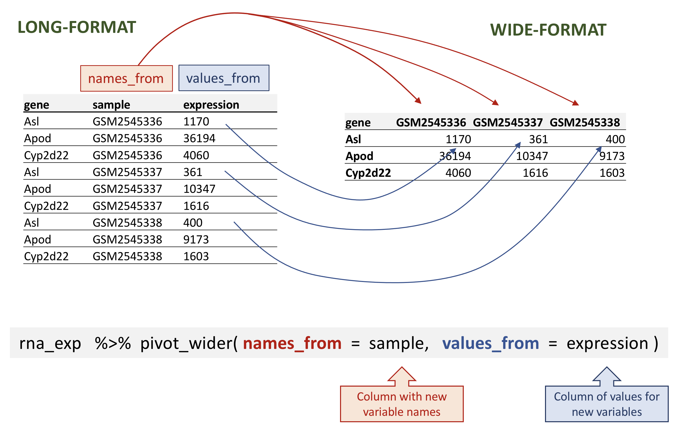— Wide pivot of the `rna` data.

R

rna_wide <- rna_exp |>
  pivot_wider(names_from = sample,
              values_from = expression)
rna_wide

输出

# A tibble: 1,474 × 23
   gene    GSM2545336 GSM2545337 GSM2545338 GSM2545339 GSM2545340 GSM2545341
   <chr>        <dbl>      <dbl>      <dbl>      <dbl>      <dbl>      <dbl>
 1 Asl           1170        361        400        586        626        988
 2 Apod         36194      10347       9173      10620      13021      29594
 3 Cyp2d22       4060       1616       1603       1901       2171       3349
 4 Klk6           287        629        641        578        448        195
 5 Fcrls           85        233        244        237        180         38
 6 Slc2a4         782        231        248        265        313        786
 7 Exd2          1619       2288       2235       2513       2366       1359
 8 Gjc2           288        595        568        551        310        146
 9 Plp1         43217     101241      96534      58354      53126      27173
10 Gnb4          1071       1791       1867       1430       1355        798
# ℹ 1,464 more rows
# ℹ 16 more variables: GSM2545342 <dbl>, GSM2545343 <dbl>, GSM2545344 <dbl>,
#   GSM2545345 <dbl>, GSM2545346 <dbl>, GSM2545347 <dbl>, GSM2545348 <dbl>,
#   GSM2545349 <dbl>, GSM2545350 <dbl>, GSM2545351 <dbl>, GSM2545352 <dbl>,
#   GSM2545353 <dbl>, GSM2545354 <dbl>, GSM2545362 <dbl>, GSM2545363 <dbl>,
#   GSM2545380 <dbl>

请注意，默认情况下，pivot_wider() 函数会为缺失值添加 NA。

假设由于某种原因，在某些样本中，部分基因的表达值缺失。在以下虚构示例中，基因 Cyp2d22 仅保留一个表达值，来自 GSM2545338 样本。

R

rna_with_missing_values <- rna |>
  select(gene, sample, expression) |>
  filter(gene %in% c("Asl", "Apod", "Cyp2d22")) |>
  filter(sample %in% c("GSM2545336", "GSM2545337", "GSM2545338")) |>
  arrange(sample) |>
  filter(!(gene == "Cyp2d22" & sample != "GSM2545338"))
rna_with_missing_values

输出

# A tibble: 7 × 3
  gene    sample     expression
  <chr>   <chr>           <dbl>
1 Asl     GSM2545336       1170
2 Apod    GSM2545336      36194
3 Asl     GSM2545337        361
4 Apod    GSM2545337      10347
5 Asl     GSM2545338        400
6 Apod    GSM2545338       9173
7 Cyp2d22 GSM2545338       1603

默认情况下，pivot_wider() 函数会为缺失值添加 NA。这可以通过 pivot_wider() 函数的 values_fill 参数进行参数化。

R

rna_with_missing_values |>
  pivot_wider(names_from = sample,
              values_from = expression)

输出

# A tibble: 3 × 4
  gene    GSM2545336 GSM2545337 GSM2545338
  <chr>        <dbl>      <dbl>      <dbl>
1 Asl           1170        361        400
2 Apod         36194      10347       9173
3 Cyp2d22         NA         NA       1603

R

rna_with_missing_values |>
  pivot_wider(names_from = sample,
              values_from = expression,
              values_fill = 0)

输出

# A tibble: 3 × 4
  gene    GSM2545336 GSM2545337 GSM2545338
  <chr>        <dbl>      <dbl>      <dbl>
1 Asl           1170        361        400
2 Apod         36194      10347       9173
3 Cyp2d22          0          0       1603

将数据转换为长格式

在另一种情况下，我们使用列名并将其转换为一对新变量。其中一个变量将列名作为值表示，另一个变量则包含此前与列名关联的值。

pivot_longer() 接收四个主要参数：

待转换的数据；
names_to：我们想要创建并填充当前列名的新列名；
values_to：我们想要创建并填充当前值的新列名；
用于填充 names_to 和 values_to 变量的列名（或用于删除的列名）。

Figure showing the long table format on the left and wide table format on the right and arrows illustrating how the column names on the left have become a new column 'sample' on the left and the values in the wide table on the right have become a new column 'expression' on the left. Below is the call to 'pivot_wider()' with annotations pointing to the 'sample', 'expression' and the '-gene' arguments. 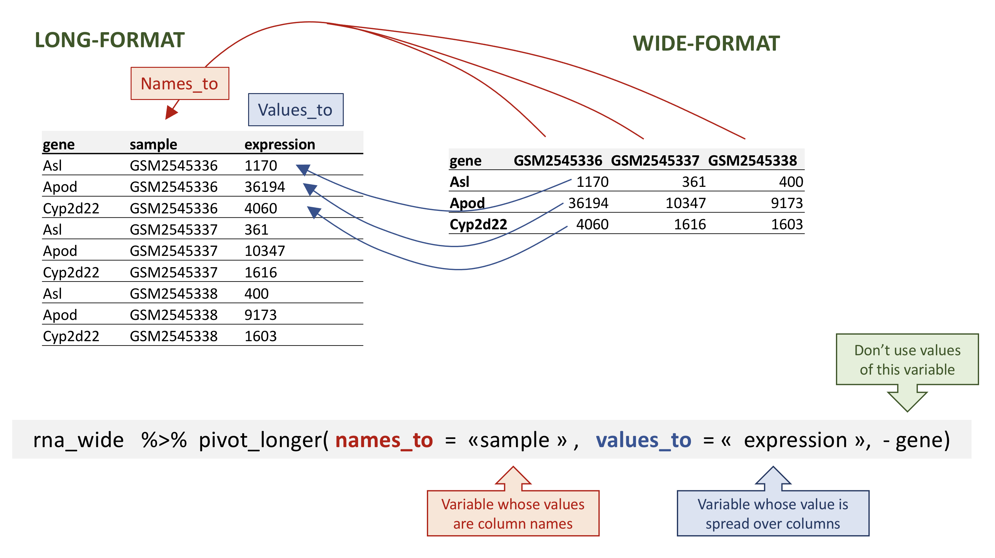— Long pivot of the `rna` data.

若要从 rna_wide 还原出 rna_long，我们将创建一个名为 sample 的键和一个名为 expression 的值，并使用除 gene 之外的所有列作为键变量。这里我们使用减号去掉 gene 列。

请注意，这里的新变量名需要加引号。

R

rna_long <- rna_wide |>
    pivot_longer(names_to = "sample",
                 values_to = "expression",
                 -gene)
rna_long

输出

# A tibble: 32,428 × 3
   gene  sample     expression
   <chr> <chr>           <dbl>
 1 Asl   GSM2545336       1170
 2 Asl   GSM2545337        361
 3 Asl   GSM2545338        400
 4 Asl   GSM2545339        586
 5 Asl   GSM2545340        626
 6 Asl   GSM2545341        988
 7 Asl   GSM2545342        836
 8 Asl   GSM2545343        535
 9 Asl   GSM2545344        586
10 Asl   GSM2545345        597
# ℹ 32,418 more rows

我们也可以使用规范来指定要包含的列。如果你有大量标识列，这种方法会很有用，因为指定要收集的列比指定要保留的列更方便。在这里，starts_with() 函数可以帮助获取样本名称，而无需逐一列出！另一种方案是使用 : 运算符！

R

rna_wide |>
    pivot_longer(names_to = "sample",
                 values_to = "expression",
                 cols = starts_with("GSM"))

输出

# A tibble: 32,428 × 3
   gene  sample     expression
   <chr> <chr>           <dbl>
 1 Asl   GSM2545336       1170
 2 Asl   GSM2545337        361
 3 Asl   GSM2545338        400
 4 Asl   GSM2545339        586
 5 Asl   GSM2545340        626
 6 Asl   GSM2545341        988
 7 Asl   GSM2545342        836
 8 Asl   GSM2545343        535
 9 Asl   GSM2545344        586
10 Asl   GSM2545345        597
# ℹ 32,418 more rows

R

rna_wide |>
    pivot_longer(names_to = "sample",
                 values_to = "expression",
                 GSM2545336:GSM2545380)

输出

# A tibble: 32,428 × 3
   gene  sample     expression
   <chr> <chr>           <dbl>
 1 Asl   GSM2545336       1170
 2 Asl   GSM2545337        361
 3 Asl   GSM2545338        400
 4 Asl   GSM2545339        586
 5 Asl   GSM2545340        626
 6 Asl   GSM2545341        988
 7 Asl   GSM2545342        836
 8 Asl   GSM2545343        535
 9 Asl   GSM2545344        586
10 Asl   GSM2545345        597
# ℹ 32,418 more rows

请注意，如果宽格式中包含缺失值，NA 将被包含在新的长格式中。

回顾我们之前那个包含缺失值的虚拟 tibble：

R

rna_with_missing_values

输出

# A tibble: 7 × 3
  gene    sample     expression
  <chr>   <chr>           <dbl>
1 Asl     GSM2545336       1170
2 Apod    GSM2545336      36194
3 Asl     GSM2545337        361
4 Apod    GSM2545337      10347
5 Asl     GSM2545338        400
6 Apod    GSM2545338       9173
7 Cyp2d22 GSM2545338       1603

R

wide_with_NA <- rna_with_missing_values |>
  pivot_wider(names_from = sample,
              values_from = expression)
wide_with_NA

输出

# A tibble: 3 × 4
  gene    GSM2545336 GSM2545337 GSM2545338
  <chr>        <dbl>      <dbl>      <dbl>
1 Asl           1170        361        400
2 Apod         36194      10347       9173
3 Cyp2d22         NA         NA       1603

R

wide_with_NA |>
    pivot_longer(names_to = "sample",
                 values_to = "expression",
                 -gene)

输出

# A tibble: 9 × 3
  gene    sample     expression
  <chr>   <chr>           <dbl>
1 Asl     GSM2545336       1170
2 Asl     GSM2545337        361
3 Asl     GSM2545338        400
4 Apod    GSM2545336      36194
5 Apod    GSM2545337      10347
6 Apod    GSM2545338       9173
7 Cyp2d22 GSM2545336         NA
8 Cyp2d22 GSM2545337         NA
9 Cyp2d22 GSM2545338       1603

转换为宽格式和长格式是一种有效的方法，可以平衡数据集，使每个重复实验的组成一致。

练习

问题

从 rna 表开始，使用 pivot_wider() 函数创建一个宽格式表，显示每只小鼠的基因表达水平。然后使用 pivot_longer() 函数还原为长格式表。

解答

R

rna1 <- rna |>
select(gene, mouse, expression) |>
pivot_wider(names_from = mouse, values_from = expression)
rna1

输出

# A tibble: 1,474 × 23
   gene     `14`    `9`  `10`  `15`  `18`   `6`   `5`  `11`  `22`  `13`  `23`
   <chr>   <dbl>  <dbl> <dbl> <dbl> <dbl> <dbl> <dbl> <dbl> <dbl> <dbl> <dbl>
 1 Asl      1170    361   400   586   626   988   836   535   586   597   938
 2 Apod    36194  10347  9173 10620 13021 29594 24959 13668 13230 15868 27769
 3 Cyp2d22  4060   1616  1603  1901  2171  3349  3122  2008  2254  2277  2985
 4 Klk6      287    629   641   578   448   195   186  1101   537   567   327
 5 Fcrls      85    233   244   237   180    38    68   375   199   177    89
 6 Slc2a4    782    231   248   265   313   786   528   249   266   357   654
 7 Exd2     1619   2288  2235  2513  2366  1359  1474  3126  2379  2173  1531
 8 Gjc2      288    595   568   551   310   146   186   791   454   370   240
 9 Plp1    43217 101241 96534 58354 53126 27173 28728 98658 61356 61647 38019
10 Gnb4     1071   1791  1867  1430  1355   798   806  2437  1394  1554   960
# ℹ 1,464 more rows
# ℹ 11 more variables: `24` <dbl>, `8` <dbl>, `7` <dbl>, `1` <dbl>, `16` <dbl>,
#   `21` <dbl>, `4` <dbl>, `2` <dbl>, `20` <dbl>, `12` <dbl>, `19` <dbl>

R

rna1 |>
pivot_longer(names_to = "mouse_id", values_to = "counts", -gene)

输出

# A tibble: 32,428 × 3
   gene  mouse_id counts
   <chr> <chr>     <dbl>
 1 Asl   14         1170
 2 Asl   9           361
 3 Asl   10          400
 4 Asl   15          586
 5 Asl   18          626
 6 Asl   6           988
 7 Asl   5           836
 8 Asl   11          535
 9 Asl   22          586
10 Asl   13          597
# ℹ 32,418 more rows

练习

问题

从 rna 数据框中提取位于 X 和 Y 染色体上的基因子集，并将该数据框展开，以 sex 为列，chromosome_name 为行，每条染色体上基因的平均表达量为值，如下所示的 tibble 所示：

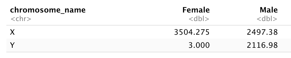
A two by two table with X and Y row names and Female and Male column names showing the total counts for each X/Y and Female/Male combination. The Y/Female combinations shows 3 counts, while all other counts are above 2000 counts.

在重塑之前，您需要先进行汇总！

解答

首先，让我们计算雄性和雌性样本中 X 和 Y 连锁基因的平均表达水平……

R

 rna |>
  filter(chromosome_name == "Y" | chromosome_name == "X") |>
  group_by(sex, chromosome_name) |>
  summarise(mean = mean(expression))

输出

`summarise()` has regrouped the output.
ℹ Summaries were computed grouped by sex and chromosome_name.
ℹ Output is grouped by sex.
ℹ Use `summarise(.groups = "drop_last")` to silence this message.
ℹ Use `summarise(.by = c(sex, chromosome_name))` for per-operation grouping
  (`?dplyr::dplyr_by`) instead.

输出

# A tibble: 4 × 3
# Groups:   sex [2]
  sex    chromosome_name  mean
  <chr>  <chr>           <dbl>
1 Female X               3504.
2 Female Y                  3
3 Male   X               2497.
4 Male   Y               2117.

并将表格转换为宽格式

R

rna_1 <- rna |>
  filter(chromosome_name == "Y" | chromosome_name == "X") |>
  group_by(sex, chromosome_name) |>
  summarise(mean = mean(expression)) |>
  pivot_wider(names_from = sex,
              values_from = mean)

输出

`summarise()` has regrouped the output.
ℹ Summaries were computed grouped by sex and chromosome_name.
ℹ Output is grouped by sex.
ℹ Use `summarise(.groups = "drop_last")` to silence this message.
ℹ Use `summarise(.by = c(sex, chromosome_name))` for per-operation grouping
  (`?dplyr::dplyr_by`) instead.

R

rna_1

输出

# A tibble: 2 × 3
  chromosome_name Female  Male
  <chr>            <dbl> <dbl>
1 X                3504. 2497.
2 Y                   3  2117.

现在将该数据框通过 pivot_longer() 进行转换，使每一行都成为一个唯一的 chromosome_name 与 gender 组合。

R

rna_1 |>
  pivot_longer(names_to = "gender",
               values_to = "mean",
               -chromosome_name)

输出

# A tibble: 4 × 3
  chromosome_name gender  mean
  <chr>           <chr>  <dbl>
1 X               Female 3504.
2 X               Male   2497.
3 Y               Female    3
4 Y               Male   2117.

练习

问题

使用 rna 数据集创建一个表达矩阵，其中每行代表基因的平均表达水平，每列代表不同的时间点。

解答

首先，让我们计算每个基因和每个时间点的平均表达量。

R

rna |>
  group_by(gene, time) |>
  summarise(mean_exp = mean(expression))

输出

`summarise()` has regrouped the output.
ℹ Summaries were computed grouped by gene and time.
ℹ Output is grouped by gene.
ℹ Use `summarise(.groups = "drop_last")` to silence this message.
ℹ Use `summarise(.by = c(gene, time))` for per-operation grouping
  (`?dplyr::dplyr_by`) instead.

输出

# A tibble: 4,422 × 3
# Groups:   gene [1,474]
   gene      time mean_exp
   <chr>    <dbl>    <dbl>
 1 AI504432     0    1034.
 2 AI504432     4    1104.
 3 AI504432     8    1014
 4 AW046200     0     155.
 5 AW046200     4     152.
 6 AW046200     8      81
 7 AW551984     0     238
 8 AW551984     4     302.
 9 AW551984     8     342.
10 Aamp         0    4603.
# ℹ 4,412 more rows

在使用 pivot_wider() 函数之前

R

rna_time <- rna |>
  group_by(gene, time) |>
  summarise(mean_exp = mean(expression)) |>
  pivot_wider(names_from = time,
              values_from = mean_exp)

输出

`summarise()` has regrouped the output.
ℹ Summaries were computed grouped by gene and time.
ℹ Output is grouped by gene.
ℹ Use `summarise(.groups = "drop_last")` to silence this message.
ℹ Use `summarise(.by = c(gene, time))` for per-operation grouping
  (`?dplyr::dplyr_by`) instead.

R

rna_time

输出

# A tibble: 1,474 × 4
# Groups:   gene [1,474]
   gene         `0`     `4`     `8`
   <chr>      <dbl>   <dbl>   <dbl>
 1 AI504432 1034.   1104.   1014
 2 AW046200  155.    152.     81
 3 AW551984  238     302.    342.
 4 Aamp     4603.   4870    4763.
 5 Abca12      5.29    4.25    4.14
 6 Abcc8    2576.   2609.   2292.
 7 Abhd14a   591.    547.    432.
 8 Abi2     4881.   4903.   4945.
 9 Abi3bp   1175.   1061.    762.
10 Abl2     2170.   2078.   2131.
# ℹ 1,464 more rows

请注意，这会生成一个部分列名以数字开头的 tibble。如果我们想选择对应于时间点的列，就不能直接使用列名……当我们选择第 4 列时会发生什么？

R

rna |>
  group_by(gene, time) |>
  summarise(mean_exp = mean(expression)) |>
  pivot_wider(names_from = time,
              values_from = mean_exp) |>
  select(gene, 4)

输出

`summarise()` has regrouped the output.
ℹ Summaries were computed grouped by gene and time.
ℹ Output is grouped by gene.
ℹ Use `summarise(.groups = "drop_last")` to silence this message.
ℹ Use `summarise(.by = c(gene, time))` for per-operation grouping
  (`?dplyr::dplyr_by`) instead.

输出

# A tibble: 1,474 × 2
# Groups:   gene [1,474]
   gene         `8`
   <chr>      <dbl>
 1 AI504432 1014
 2 AW046200   81
 3 AW551984  342.
 4 Aamp     4763.
 5 Abca12      4.14
 6 Abcc8    2292.
 7 Abhd14a   432.
 8 Abi2     4945.
 9 Abi3bp    762.
10 Abl2     2131.
# ℹ 1,464 more rows

若要选择时间点 4，我们需要使用反引号 “`” 来引号包裹列名。

R

rna |>
  group_by(gene, time) |>
  summarise(mean_exp = mean(expression)) |>
  pivot_wider(names_from = time,
              values_from = mean_exp) |>
  select(gene, `4`)

输出

`summarise()` has regrouped the output.
ℹ Summaries were computed grouped by gene and time.
ℹ Output is grouped by gene.
ℹ Use `summarise(.groups = "drop_last")` to silence this message.
ℹ Use `summarise(.by = c(gene, time))` for per-operation grouping
  (`?dplyr::dplyr_by`) instead.

输出

# A tibble: 1,474 × 2
# Groups:   gene [1,474]
   gene         `4`
   <chr>      <dbl>
 1 AI504432 1104.
 2 AW046200  152.
 3 AW551984  302.
 4 Aamp     4870
 5 Abca12      4.25
 6 Abcc8    2609.
 7 Abhd14a   547.
 8 Abi2     4903.
 9 Abi3bp   1061.
10 Abl2     2078.
# ℹ 1,464 more rows

另一种方案是重命名该列，选择一个不以数字开头的名称：

R

rna |>
  group_by(gene, time) |>
  summarise(mean_exp = mean(expression)) |>
  pivot_wider(names_from = time,
              values_from = mean_exp) |>
  rename("time0" = `0`, "time4" = `4`, "time8" = `8`) |>
  select(gene, time4)

输出

`summarise()` has regrouped the output.
ℹ Summaries were computed grouped by gene and time.
ℹ Output is grouped by gene.
ℹ Use `summarise(.groups = "drop_last")` to silence this message.
ℹ Use `summarise(.by = c(gene, time))` for per-operation grouping
  (`?dplyr::dplyr_by`) instead.

输出

# A tibble: 1,474 × 2
# Groups:   gene [1,474]
   gene       time4
   <chr>      <dbl>
 1 AI504432 1104.
 2 AW046200  152.
 3 AW551984  302.
 4 Aamp     4870
 5 Abca12      4.25
 6 Abcc8    2609.
 7 Abhd14a   547.
 8 Abi2     4903.
 9 Abi3bp   1061.
10 Abl2     2078.
# ℹ 1,464 more rows

练习

问题

使用之前包含每个时间点平均表达水平的数据框，创建一个新列，其中包含时间点 8 与时间点 0 之间的倍数变化，以及时间点 8 与时间点 4 之间的倍数变化。将此表转换为长格式表，汇总计算出的倍数变化。

解答

从 rna_time tibble 开始：

R

rna_time

输出

# A tibble: 1,474 × 4
# Groups:   gene [1,474]
   gene         `0`     `4`     `8`
   <chr>      <dbl>   <dbl>   <dbl>
 1 AI504432 1034.   1104.   1014
 2 AW046200  155.    152.     81
 3 AW551984  238     302.    342.
 4 Aamp     4603.   4870    4763.
 5 Abca12      5.29    4.25    4.14
 6 Abcc8    2576.   2609.   2292.
 7 Abhd14a   591.    547.    432.
 8 Abi2     4881.   4903.   4945.
 9 Abi3bp   1175.   1061.    762.
10 Abl2     2170.   2078.   2131.
# ℹ 1,464 more rows

计算倍数变化：

R

rna_time |>
  mutate(time_8_vs_0 = `8` / `0`, time_8_vs_4 = `8` / `4`)

输出

# A tibble: 1,474 × 6
# Groups:   gene [1,474]
   gene         `0`     `4`     `8` time_8_vs_0 time_8_vs_4
   <chr>      <dbl>   <dbl>   <dbl>       <dbl>       <dbl>
 1 AI504432 1034.   1104.   1014          0.981       0.918
 2 AW046200  155.    152.     81          0.522       0.532
 3 AW551984  238     302.    342.         1.44        1.13
 4 Aamp     4603.   4870    4763.         1.03        0.978
 5 Abca12      5.29    4.25    4.14       0.784       0.975
 6 Abcc8    2576.   2609.   2292.         0.889       0.878
 7 Abhd14a   591.    547.    432.         0.731       0.791
 8 Abi2     4881.   4903.   4945.         1.01        1.01
 9 Abi3bp   1175.   1061.    762.         0.649       0.719
10 Abl2     2170.   2078.   2131.         0.982       1.03
# ℹ 1,464 more rows

并使用 pivot_longer() 函数：

R

rna_time |>
  mutate(time_8_vs_0 = `8` / `0`, time_8_vs_4 = `8` / `4`) |>
  pivot_longer(names_to = "comparisons",
               values_to = "Fold_changes",
               time_8_vs_0:time_8_vs_4)

输出

# A tibble: 2,948 × 6
# Groups:   gene [1,474]
   gene         `0`     `4`     `8` comparisons Fold_changes
   <chr>      <dbl>   <dbl>   <dbl> <chr>              <dbl>
 1 AI504432 1034.   1104.   1014    time_8_vs_0        0.981
 2 AI504432 1034.   1104.   1014    time_8_vs_4        0.918
 3 AW046200  155.    152.     81    time_8_vs_0        0.522
 4 AW046200  155.    152.     81    time_8_vs_4        0.532
 5 AW551984  238     302.    342.   time_8_vs_0        1.44
 6 AW551984  238     302.    342.   time_8_vs_4        1.13
 7 Aamp     4603.   4870    4763.   time_8_vs_0        1.03
 8 Aamp     4603.   4870    4763.   time_8_vs_4        0.978
 9 Abca12      5.29    4.25    4.14 time_8_vs_0        0.784
10 Abca12      5.29    4.25    4.14 time_8_vs_4        0.975
# ℹ 2,938 more rows

连接表

在许多实际场景中，数据分布在多个表格中。这通常是因为不同类型的信息是从不同的来源收集的。

在某些分析中，可能需要根据一个所有表格共有的列，将两个或多个表格的数据合并为一个数据框。

dplyr 包提供了一组连接函数，用于根据指定列中的匹配项将两个数据框合并。在此，我们将简要介绍连接操作。如需进一步阅读，请参阅关于表连接的章节。数据转换速查表也提供了关于表连接的简要概述。

我们将使用一个小表 rna_mini 来演示连接操作，该表我们将通过对原始表 rna 进行子集提取，仅保留 3 列和 10 行来创建。

R

rna_mini <- rna |>
   select(gene, sample, expression) |>
   head(10)
rna_mini

输出

# A tibble: 10 × 3
   gene    sample     expression
   <chr>   <chr>           <dbl>
 1 Asl     GSM2545336       1170
 2 Apod    GSM2545336      36194
 3 Cyp2d22 GSM2545336       4060
 4 Klk6    GSM2545336        287
 5 Fcrls   GSM2545336         85
 6 Slc2a4  GSM2545336        782
 7 Exd2    GSM2545336       1619
 8 Gjc2    GSM2545336        288
 9 Plp1    GSM2545336      43217
10 Gnb4    GSM2545336       1071

第二张表 annot1 包含 2 列：gene 和 gene_description。您可以点击链接下载 annot1.csv 并将其移至 data/ 文件夹，或者使用下面的 R 代码将其直接下载到该文件夹。

R

download.file(url = "https://carpentries-incubator.github.io/bioc-intro/data/annot1.csv",
              destfile = "data/annot1.csv")
annot1 <- read_csv(file = "data/annot1.csv")
annot1

输出

# A tibble: 10 × 2
   gene    gene_description
   <chr>   <chr>
 1 Cyp2d22 cytochrome P450, family 2, subfamily d, polypeptide 22 [Source:MGI S…
 2 Klk6    kallikrein related-peptidase 6 [Source:MGI Symbol;Acc:MGI:1343166]
 3 Fcrls   Fc receptor-like S, scavenger receptor [Source:MGI Symbol;Acc:MGI:19…
 4 Plp1    proteolipid protein (myelin) 1 [Source:MGI Symbol;Acc:MGI:97623]
 5 Exd2    exonuclease 3'-5' domain containing 2 [Source:MGI Symbol;Acc:MGI:192…
 6 Apod    apolipoprotein D [Source:MGI Symbol;Acc:MGI:88056]
 7 Gnb4    guanine nucleotide binding protein (G protein), beta 4 [Source:MGI S…
 8 Slc2a4  solute carrier family 2 (facilitated glucose transporter), member 4 …
 9 Asl     argininosuccinate lyase [Source:MGI Symbol;Acc:MGI:88084]
10 Gjc2    gap junction protein, gamma 2 [Source:MGI Symbol;Acc:MGI:2153060]

现在，我们想使用 dplyr 包中的 full_join() 函数将这两个表合并为一个包含所有变量的表。该函数会自动寻找公共变量，以匹配第一张表和第二张表的列。在本例中，gene 就是公共变量。这类变量被称为键。键用于在不同表之间匹配观测值。

R

full_join(rna_mini, annot1)

输出

Joining with `by = join_by(gene)`

输出

# A tibble: 10 × 4
   gene    sample     expression gene_description
   <chr>   <chr>           <dbl> <chr>
 1 Asl     GSM2545336       1170 argininosuccinate lyase [Source:MGI Symbol;Acc…
 2 Apod    GSM2545336      36194 apolipoprotein D [Source:MGI Symbol;Acc:MGI:88…
 3 Cyp2d22 GSM2545336       4060 cytochrome P450, family 2, subfamily d, polype…
 4 Klk6    GSM2545336        287 kallikrein related-peptidase 6 [Source:MGI Sym…
 5 Fcrls   GSM2545336         85 Fc receptor-like S, scavenger receptor [Source…
 6 Slc2a4  GSM2545336        782 solute carrier family 2 (facilitated glucose t…
 7 Exd2    GSM2545336       1619 exonuclease 3'-5' domain containing 2 [Source:…
 8 Gjc2    GSM2545336        288 gap junction protein, gamma 2 [Source:MGI Symb…
 9 Plp1    GSM2545336      43217 proteolipid protein (myelin) 1 [Source:MGI Sym…
10 Gnb4    GSM2545336       1071 guanine nucleotide binding protein (G protein)…

在实际应用中，基因注释有时会采用不同的标注方式。

annot2 表与 annot1 完全相同，仅将包含基因名称的变量标注不同。同样，您可以自行下载 annot2.csv 并将其移至 data/，或者使用下面的 R 代码。

R

download.file(url = "https://carpentries-incubator.github.io/bioc-intro/data/annot2.csv",
              destfile = "data/annot2.csv")
annot2 <- read_csv(file = "data/annot2.csv")
annot2

输出

# A tibble: 10 × 2
   external_gene_name description
   <chr>              <chr>
 1 Cyp2d22            cytochrome P450, family 2, subfamily d, polypeptide 22 [S…
 2 Klk6               kallikrein related-peptidase 6 [Source:MGI Symbol;Acc:MGI…
 3 Fcrls              Fc receptor-like S, scavenger receptor [Source:MGI Symbol…
 4 Plp1               proteolipid protein (myelin) 1 [Source:MGI Symbol;Acc:MGI…
 5 Exd2               exonuclease 3'-5' domain containing 2 [Source:MGI Symbol;…
 6 Apod               apolipoprotein D [Source:MGI Symbol;Acc:MGI:88056]
 7 Gnb4               guanine nucleotide binding protein (G protein), beta 4 [S…
 8 Slc2a4             solute carrier family 2 (facilitated glucose transporter)…
 9 Asl                argininosuccinate lyase [Source:MGI Symbol;Acc:MGI:88084]
10 Gjc2               gap junction protein, gamma 2 [Source:MGI Symbol;Acc:MGI:…

如果没有任何变量名匹配，我们可以手动设置用于匹配的变量。这些变量可以通过 by 参数来设置，如下面 rna_mini 和 annot2 表所示。

R

full_join(rna_mini, annot2, by = c("gene" = "external_gene_name"))

输出

# A tibble: 10 × 4
   gene    sample     expression description
   <chr>   <chr>           <dbl> <chr>
 1 Asl     GSM2545336       1170 argininosuccinate lyase [Source:MGI Symbol;Acc…
 2 Apod    GSM2545336      36194 apolipoprotein D [Source:MGI Symbol;Acc:MGI:88…
 3 Cyp2d22 GSM2545336       4060 cytochrome P450, family 2, subfamily d, polype…
 4 Klk6    GSM2545336        287 kallikrein related-peptidase 6 [Source:MGI Sym…
 5 Fcrls   GSM2545336         85 Fc receptor-like S, scavenger receptor [Source…
 6 Slc2a4  GSM2545336        782 solute carrier family 2 (facilitated glucose t…
 7 Exd2    GSM2545336       1619 exonuclease 3'-5' domain containing 2 [Source:…
 8 Gjc2    GSM2545336        288 gap junction protein, gamma 2 [Source:MGI Symb…
 9 Plp1    GSM2545336      43217 proteolipid protein (myelin) 1 [Source:MGI Sym…
10 Gnb4    GSM2545336       1071 guanine nucleotide binding protein (G protein)…

如上所示，第一个表的变量名在合并后的表中得以保留。

练习

挑战：

点击此链接下载 annot3 表，并将该表放入你的 data/ 存储库中。使用 full_join() 函数，将 rna_mini 和 annot3 表进行连接。基因 Klk6、mt-Tf、mt-Rnr1、mt-Tv、mt-Rnr2 和 mt-Tl1 发生了什么变化？

解答

R

annot3 <- read_csv("data/annot3.csv")
full_join(rna_mini, annot3)

输出

# A tibble: 15 × 4
   gene    sample     expression gene_description
   <chr>   <chr>           <dbl> <chr>
 1 Asl     GSM2545336       1170 argininosuccinate lyase [Source:MGI Symbol;Acc…
 2 Apod    GSM2545336      36194 apolipoprotein D [Source:MGI Symbol;Acc:MGI:88…
 3 Cyp2d22 GSM2545336       4060 cytochrome P450, family 2, subfamily d, polype…
 4 Klk6    GSM2545336        287 <NA>
 5 Fcrls   GSM2545336         85 Fc receptor-like S, scavenger receptor [Source…
 6 Slc2a4  GSM2545336        782 solute carrier family 2 (facilitated glucose t…
 7 Exd2    GSM2545336       1619 exonuclease 3'-5' domain containing 2 [Source:…
 8 Gjc2    GSM2545336        288 gap junction protein, gamma 2 [Source:MGI Symb…
 9 Plp1    GSM2545336      43217 proteolipid protein (myelin) 1 [Source:MGI Sym…
10 Gnb4    GSM2545336       1071 guanine nucleotide binding protein (G protein)…
11 mt-Tf   <NA>               NA mitochondrially encoded tRNA phenylalanine [So…
12 mt-Rnr1 <NA>               NA mitochondrially encoded 12S rRNA [Source:MGI S…
13 mt-Tv   <NA>               NA mitochondrially encoded tRNA valine [Source:MG…
14 mt-Rnr2 <NA>               NA mitochondrially encoded 16S rRNA [Source:MGI S…
15 mt-Tl1  <NA>               NA mitochondrially encoded tRNA leucine 1 [Source…

基因 Klk6 仅存在于 rna_mini 中，而基因 mt-Tf、mt-Rnr1、mt-Tv、mt-Rnr2 和 mt-Tl1 仅存在于 annot3 表中。它们在该表变量中的相应值均被编码为缺失值。

导出数据

既然您已经学会了如何使用 dplyr 从原始数据中提取信息或进行汇总，您可能想要导出这些新数据集，以便与合作者共享或用于存档。

与用于将 CSV 文件读取到 R 中的 read_csv() 函数类似，还有一个 write_csv() 函数可从数据框生成 CSV 文件。

在使用 write_csv() 之前，我们将在工作目录中创建一个新文件夹 data_output，用于存储此生成的数据集。我们不希望将生成的数据集写入与原始数据相同的目录中。将两者分开存放是一个良好的实践。data 文件夹应仅包含原始且未经修改的数据，且应保持原样，以确保不会将其删除或修改。相比之下，我们的脚本将生成 data_output 文件夹中的内容，因此即使其中的文件被删除，我们也始终可以重新生成它们。

让我们使用 write_csv() 来保存我们之前创建的 rna_wide 表格。

R

write_csv(rna_wide, file = "data_output/rna_wide.csv")

要点

使用 tidyverse 元包在 R 中处理表格数据

使用 dplyr 处理和分析数据

概述

问题

学习目标

使用 dplyr 和 tidyr 进行数据处理

R

R

使用 tidyverse 加载数据

R

输出

选择列与过滤行

R

输出

R

输出

R

输出

R

输出

R

输出

R

输出

R

输出

管道

R

输出

R

输出

R

输出

R

输出

挑战：

解答

R

输出

创建和修改列（mutate）

R

输出

R

输出

挑战

解答

R

输出

分-应用-合并数据分析

R

输出

R

输出

summarise() 函数

R

输出

R

输出

R

输出

输出

R

输出

输出

挑战

解答

R

输出

计数

R

输出

R

输出

R

输出

R

输出

输出

R

输出

R

使用 `dplyr` 和 `tidyr` 进行数据处理

`summarise()` 函数