
数据可视化
最后更新于 2026-11-07 | 编辑此页
概述
问题
- R 中的可视化
学习目标
- 使用 ggplot 绘制散点图、箱线图、折线图等。
- 设置通用图表设置。
- 描述什么是分面,并在 ggplot 中应用分面。
- 修改现有 ggplot 图表的视觉效果(包括轴标签和颜色)。
- 利用数据框中的数据构建复杂且定制化的图表。
本集基于 Data Carpentries 的 Data Analysis and Visualisation in R for Ecologists 课程。
数据可视化
我们首先加载所需的包。ggplot2 包含在
tidyverse 包中。
R
library("tidyverse")
如果工作区中已没有这些数据,请重新加载我们在上一课中保存的数据。
R
rna <- read.csv("data/rnaseq.csv")
数据可视化速查表将涵盖
ggplot2
的基础知识和更高级的功能,并在起到提醒作用的同时,帮助您概览该包中提供的多种数据表示方式。Thomas
Lin Pedersen 提供的以下视频教程(第一部分 和 第二部分)也非常有参考价值。
使用 ggplot2 绘图
ggplot2
是一个绘图包,能够轻松地利用数据框中的数据创建复杂的图表。它提供了一种更具程序化的接口,用于指定要绘制的变量、显示方式以及通用的视觉属性。支撑
ggplot2 的理论基础是“图形语法”(Grammar of
Graphics, Wilkinson (2005)
)。采用这种方法,即使底层数据发生变化,或者我们决定将柱状图改为散点图,也仅需进行极少的修改。这有助于在最少的调整和微调下,创建出发表级质量的图表。
有一本关于 ggplot2 ( Wickham
(2016) ) 的书,提供了很好的概览,但已过时。第三版正在筹备中,将在网上免费提供。ggplot2
网页 (https://ggplot2.tidyverse.org)
提供了丰富的文档。
ggplot2
函数适用于“长格式”数据,即每个维度对应一列,每个观测值对应一行。结构良好的数据将在使用
ggplot2 绘制图表时为你节省大量时间。
ggplot 图形是通过逐步添加新元素来构建的。以这种方式添加图层,可以为图表提供极大的灵活性和自定义能力。
图形语法(Grammar of Graphics)的核心思想是,你可以用相同的 3 个组件构建任何图表:(1) 数据集,(2) 坐标系,以及 (3) geoms —— 即表示数据点的视觉标记 1
要构建 ggplot,我们将使用以下基本模板,该模板适用于不同类型的图表:
ggplot(data = <DATA>, mapping = aes(<MAPPINGS>)) + <GEOM_FUNCTION>()- 使用
ggplot()函数,并通过data参数将图表绑定到特定的 数据框 中
R
ggplot(data = rna)
- 定义一个映射(使用 aesthetic (
aes) 函数),通过选择要绘制的变量并指定在图表中如何呈现它们,例如作为 x/y 坐标,或作为尺寸、形状、颜色等特性。
R
ggplot(data = rna, mapping = aes(x = expression))
-
添加“geoms”——几何图形,即图表中数据的图形表示(点、线、柱)。
ggplot2提供了许多不同的 geoms;今天我们将使用一些常用的,包括:* `geom_point()` for scatter plots, dot plots, etc. * `geom_histogram()` for histograms * `geom_boxplot()` for, well, boxplots! * `geom_line()` for trend lines, time series, etc.
若要在图表中添加几何对象 (geometry),请使用 +
运算符。让我们先使用 geom_histogram():
R
ggplot(data = rna, mapping = aes(x = expression)) +
  geom_histogram()
输出
`stat_bin()` using `bins = 30`. Pick better value `binwidth`.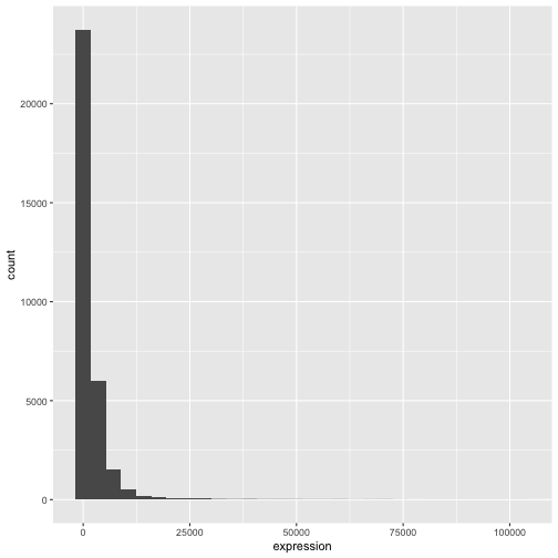
ggplot2 包中的 +
尤为实用,因为它允许你修改现有的 ggplot
对象。这意味着你可以轻松地设置图表模板,并便捷地探索不同类型的图表,因此上述图表也可以通过如下代码生成:
R
# Assign plot to a variable
rna_plot <- ggplot(data = rna,
                   mapping = aes(x = expression))

# Draw the plot
rna_plot + geom_histogram()
挑战
你可能已经注意到,在绘制直方图时会出现一条自动提示信息:
输出
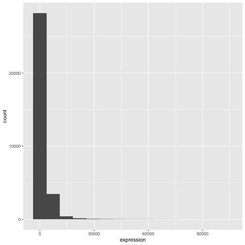
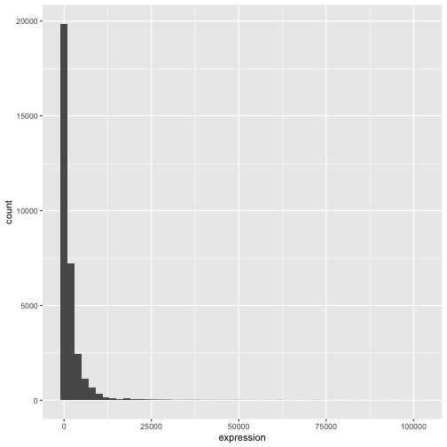
`stat_bin()` using `bins = 30`. Pick better value `binwidth`.修改 geom_histogram() 的参数 bins 或
binwidth 以更改分箱数或宽度。
R
# change bins
ggplot(rna, aes(x = expression)) +
    geom_histogram(bins = 15)
R
# change binwidth
ggplot(rna, aes(x = expression)) +
    geom_histogram(binwidth = 2000)
我们可以看到,数据向右偏。我们可以进行以2为底的对数变换,以获得更对称的分布。请注意,我们在此添加了一个小的常数值
(+1),以避免在表达值为 0 时返回 -Inf 值。
R
rna <- rna |>
  mutate(expression_log = log2(expression + 1))
现在如果绘制以2为底的对数变换后的表达量直方图,分布确实更接近正态分布。
R
ggplot(rna, aes(x = expression_log)) + geom_histogram()
输出
`stat_bin()` using `bins = 30`. Pick better value `binwidth`.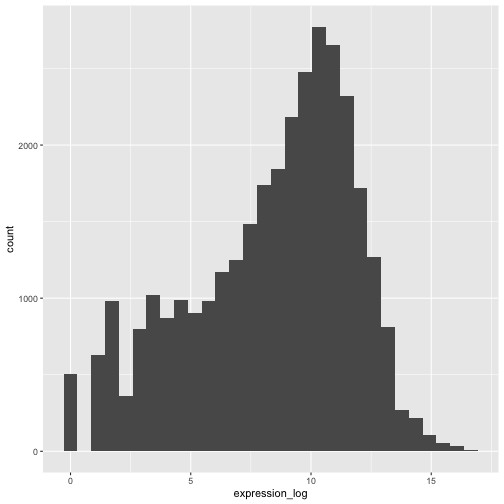
接下来,我们将处理以对数变换后的表达量值。
挑战
另一种可视化此变换的方法是考虑观测值的尺度。例如,调整轴的尺度可能有助于更好地分布观测值在图表空间中。调整轴尺度的方法与添加/修改其他组件类似(即通过逐步添加命令)。请尝试进行此项修改:
- 以 log10 尺度表示未经变换的表达量;参见
scale_x_log10()。将其与之前的图表进行对比。为什么现在会出现警告信息?
R
ggplot(data = rna,mapping = aes(x = expression))+
  geom_histogram() +
  scale_x_log10()
警告
Warning in scale_x_log10(): log-10 transformation introduced infinite values.输出
`stat_bin()` using `bins = 30`. Pick better value `binwidth`.警告
Warning: Removed 507 rows containing non-finite outside the scale range
(`stat_bin()`).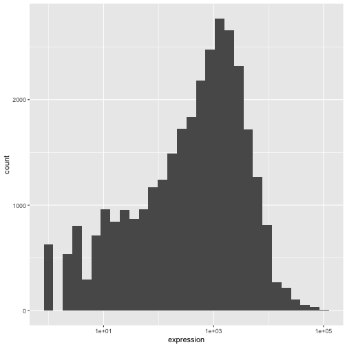
注释
- 在
ggplot()函数中指定的设置可由随后添加的任何 geom 图层继承(即这些是全局绘图设置),包括在aes()中设置的 x 轴和 y 轴映射。 - 您还可以为特定的 geom 指定映射,而无需依赖于
ggplot()函数中定义的全局映射。 - 用于添加新图层的
+符号必须放置在包含前一个图层的行末尾。如果相反,将+符号添加到包含新图层的行首,ggplot2将不会添加该新图层,并返回错误消息。
R
# This is the correct syntax for adding layers
rna_plot +
  geom_histogram()

# This will not add the new layer and will return an error message
rna_plot
  + geom_histogram()
迭代构建图表
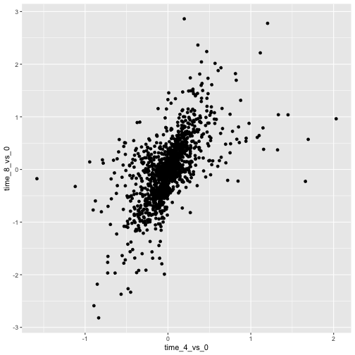
现在我们将使用 geom_point()
函数绘制一个包含两个连续变量的散点图。该图将表示时间 8 与时间 0 以及时间
4 与时间 0
之间表达量的以2为底的对数倍数变化。为此,我们首先需要计算每个基因和时间点的对数变换后的表达量值的平均值,然后通过减去时间
8 与时间 0 以及时间 4 与时间 0
之间对数表达量的平均值,来计算对数倍数变化。请注意,我们在此还包含了稍后用于表示基因的基因生物型。我们将把倍数变化保存到一个名为
rna_fc. 的新数据框中。
R
rna_fc <- rna |> select(gene, time,
                         gene_biotype, expression_log) |>
  group_by(gene, time, gene_biotype) |>
  summarize(mean_exp = mean(expression_log)) |>
  pivot_wider(names_from = time,
              values_from = mean_exp) |>
  mutate(time_8_vs_0 = `8` - `0`, time_4_vs_0 = `4` - `0`)
输出
`summarise()` has regrouped the output.
ℹ Summaries were computed grouped by gene, time, and gene_biotype.
ℹ Output is grouped by gene and time.
ℹ Use `summarise(.groups = "drop_last")` to silence this message.
ℹ Use `summarise(.by = c(gene, time, gene_biotype))` for per-operation grouping
  (`?dplyr::dplyr_by`) instead.
接下来,我们可以使用新创建的数据集 rna_fc 构建一个
ggplot。使用 ggplot2
构建图表通常是一个迭代过程。我们首先定义要使用的数据集,布置轴,并选择一个
geom:
R
ggplot(data = rna_fc, mapping = aes(x = time_4_vs_0, y = time_8_vs_0)) +
  geom_point()
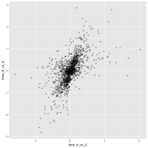
然后,我们开始修改这张图,以从中提取更多信息。例如,我们可以添加透明度
(alpha) 以避免重叠:
R
ggplot(data = rna_fc, mapping = aes(x = time_4_vs_0, y = time_8_vs_0)) +
  geom_point(alpha = 0.3)
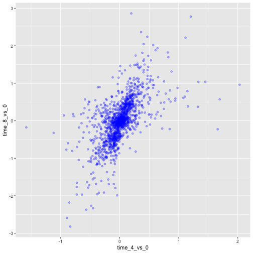
我们还可以为所有点添加颜色:
R
ggplot(data = rna_fc, mapping = aes(x = time_4_vs_0, y = time_8_vs_0)) +
  geom_point(alpha = 0.3, color = "blue")
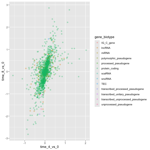
或者,若要为图中的每个基因着色,可以将向量作为参数
color 的输入。ggplot2
将提供与向量中不同值相对应的不同颜色。以下是一个使用
gene_biotype 进行着色的示例:
R
ggplot(data = rna_fc, mapping = aes(x = time_4_vs_0, y = time_8_vs_0)) +
  geom_point(alpha = 0.3, aes(color = gene_biotype))
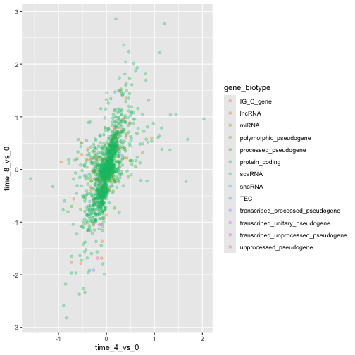
我们也可以直接在 ggplot() 函数提供的映射中指定颜色。任何
geom 图层都将看到这些颜色,且映射将由 aes() 中设置的 x 轴和
y 轴决定。
R
ggplot(data = rna_fc, mapping = aes(x = time_4_vs_0, y = time_8_vs_0,
                                color = gene_biotype)) +
  geom_point(alpha = 0.3)
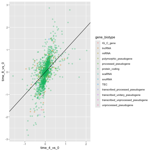
最后,我们还可以使用 geom_abline()
函数添加一条对角线:
R
ggplot(data = rna_fc, mapping = aes(x = time_4_vs_0, y = time_8_vs_0,
                                color = gene_biotype)) +
  geom_point(alpha = 0.3) +
  geom_abline(intercept = 0)
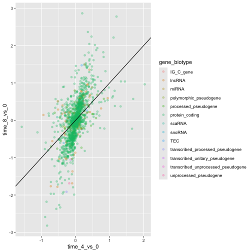
请注意,我们可以将 geom 图层从 geom_point 更改为
geom_jitter,而颜色仍将由 gene_biotype
决定。
R
ggplot(data = rna_fc, mapping = aes(x = time_4_vs_0, y = time_8_vs_0,
                                color = gene_biotype)) +
  geom_jitter(alpha = 0.3) +
  geom_abline(intercept = 0)
挑战
散点图是处理小规模数据集的实用探索工具。对于像 rna_fc
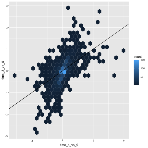
数据集这样包含大量观测值的数据集,点的重叠可能是散点图的局限性。处理此类场景的一种策略是对观测值进行六边形分箱。图表空间被镶嵌成六边形。每个六边形根据其边界内观测值的数量被赋予一个颜色。
若要在
ggplot2中使用六边形分箱法,请先从 CRAN 安装 R 包hexbin并加载它。然后使用
geom_hex()函数生成 hexbin 图表。与散点图相比,六边形分箱图的相对优缺点是什么?请查看上述散点图,并将其与你创建的六边形分箱图进行对比。
R
install.packages("hexbin")
R
library("hexbin")

ggplot(data = rna_fc, mapping = aes(x = time_4_vs_0, y = time_8_vs_0)) +
  geom_hex() +
  geom_abline(intercept = 0)
挑战
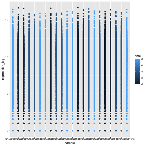
利用刚才学到的知识,为 rna 数据集绘制
expression_log 与 sample
的散点图,并用不同颜色表示时间。这是否是展示此类数据的好方法?
R
ggplot(data = rna, mapping = aes(y = expression_log, x = sample)) +
    geom_point(aes(color = time))
箱线图
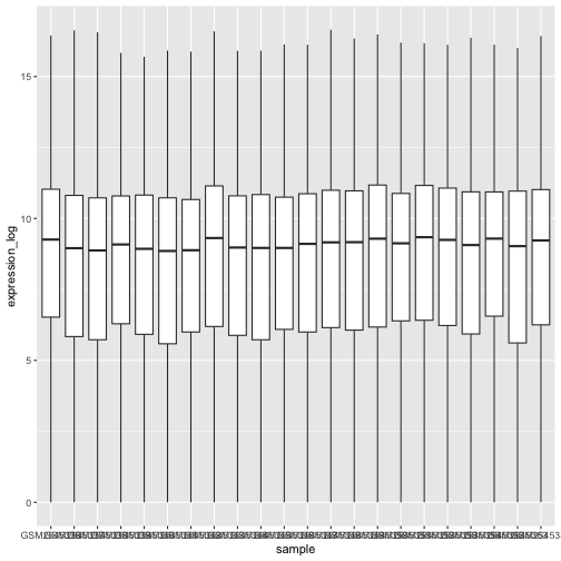
我们可以使用箱线图来可视化每个样本中基因表达的分布:
R
ggplot(data = rna,
         mapping = aes(y = expression_log, x = sample)) +
  geom_boxplot()
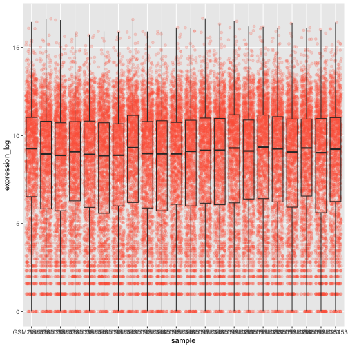
通过在箱线图中添加点,我们可以更清晰地了解测量值的数量及其分布情况:
R
ggplot(data = rna,
         mapping = aes(y = expression_log, x = sample)) +
  geom_jitter(alpha = 0.2, color = "tomato") +
  geom_boxplot(alpha = 0)
挑战
请注意,箱线图层位于抖动层之上。你需要修改代码中的哪些部分,才能将箱线图置于点图下方?
我们应该调换这两个 geom 的顺序:
R
ggplot(data = rna,
         mapping = aes(y = expression_log, x = sample)) +
  geom_boxplot(alpha = 0) +
  geom_jitter(alpha = 0.2, color = "tomato")
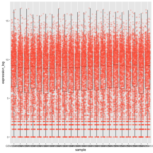
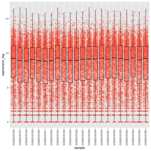
你可能会注意到 x 轴上的数值仍然无法清晰读取。让我们更改标签的方向,并对其进行垂直和水平调整,以免重叠。你可以使用 90 度角,或者通过尝试来找到斜向标签的合适角度:
R
ggplot(data = rna,
         mapping = aes(y = expression_log, x = sample)) +
  geom_jitter(alpha = 0.2, color = "tomato") +
  geom_boxplot(alpha = 0) +
  theme(axis.text.x = element_text(angle = 90,  hjust = 0.5, vjust = 0.5))
挑战
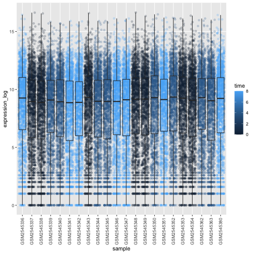
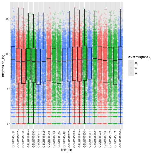
根据感染时长 (time) 为箱线图上的数据点添加颜色。
提示: 检查 time 的类型。考虑直接在 ggplot
映射中将 time 的类型从整数改为因子。为什么这种改变会影响 R
绘制图表的方式?
R
# time as integer
ggplot(data = rna,
         mapping = aes(y = expression_log,
                       x = sample)) +
  geom_jitter(alpha = 0.2, aes(color = time)) +
  geom_boxplot(alpha = 0) +
  theme(axis.text.x = element_text(angle = 90,  hjust = 0.5, vjust = 0.5))
R
# time as factor
ggplot(data = rna,
         mapping = aes(y = expression_log,
                       x = sample)) +
  geom_jitter(alpha = 0.2, aes(color = as.factor(time))) +
  geom_boxplot(alpha = 0) +
  theme(axis.text.x = element_text(angle = 90,  hjust = 0.5, vjust = 0.5))
挑战
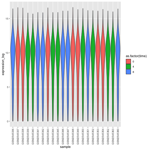
箱线图是有用的汇总图,但会掩盖分布的形状。例如,如果分布呈双峰分布,我们在箱线图中无法看到这一点。箱线图的另一种替代方案是小提琴图,它会绘制出形状(点的密度)。
- 将箱线图替换为小提琴图;参见
geom_violin()。根据时间使用参数fill填充小提琴图。
R
ggplot(data = rna,
         mapping = aes(y = expression_log, x = sample)) +
  geom_violin(aes(fill = as.factor(time))) +
  theme(axis.text.x = element_text(angle = 90,  hjust = 0.5, vjust = 0.5))
挑战
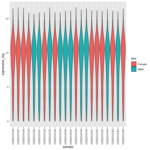
- 修改小提琴图,以
sex填充小提琴。
R
ggplot(data = rna,
         mapping = aes(y = expression_log, x = sample)) +
  geom_violin(aes(fill = sex)) +
  theme(axis.text.x = element_text(angle = 90,  hjust = 0.5, vjust = 0.5))
折线图
让我们计算这 10 个对比时间 8 与时间 0
时以2为底的对数倍数变化最大的基因,其每个感染时长的平均表达量。首先,我们需要选择这些基因,并创建一个包含这
10 个选定基因的 rna 子集
sub_rna,然后我们需要对数据进行分组,并计算每个组内的平均基因表达量:
R
rna_fc <- rna_fc |> arrange(desc(time_8_vs_0))

genes_selected <- rna_fc$gene[1:10]

sub_rna <- rna |>
    filter(gene %in% genes_selected)

mean_exp_by_time <- sub_rna |>
  group_by(gene,time) |>
    summarize(mean_exp = mean(expression_log))
输出
`summarise()` has regrouped the output.
ℹ Summaries were computed grouped by gene and time.
ℹ Output is grouped by gene.
ℹ Use `summarise(.groups = "drop_last")` to silence this message.
ℹ Use `summarise(.by = c(gene, time))` for per-operation grouping
  (`?dplyr::dplyr_by`) instead.
R
mean_exp_by_time
输出
# A tibble: 30 × 3
# Groups:   gene [10]
   gene   time mean_exp
   <chr> <int>    <dbl>
 1 Acr       0     5.07
 2 Acr       4     5.54
 3 Acr       8     7.31
 4 Aipl1     0     3.70
 5 Aipl1     4     3.89
 6 Aipl1     8     6.56
 7 Bst1      0     3.20
 8 Bst1      4     3.77
 9 Bst1      8     5.22
10 Chil3     0     4.00
# ℹ 20 more rows
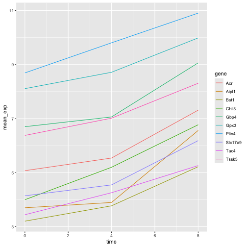
我们可以绘制一张线图,将感染时长作为 x 轴,将平均表达量作为 y 轴:
R
ggplot(data = mean_exp_by_time, mapping = aes(x = time, y = mean_exp)) +
  geom_line()
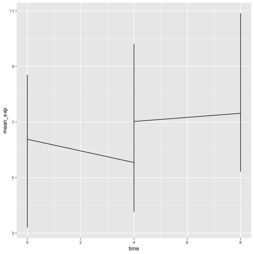
遗憾的是,这行不通,因为我们将所有基因的数据一起绘制了。我们需要通过修改
aesthetic 函数以包含 group = gene,来告诉 ggplot
为每个基因绘制一条线:
R
ggplot(data = mean_exp_by_time,
       mapping = aes(x = time, y = mean_exp, group = gene)) +
  geom_line()
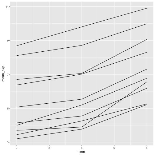
如果我们添加颜色,就能在图表中区分不同的基因(使用 color
还会自动对数据进行分组):
R
ggplot(data = mean_exp_by_time,
       mapping = aes(x = time, y = mean_exp, color = gene)) +
  geom_line()
分面
ggplot2 有一种名为 faceting
的特殊技术,允许用户根据数据集中包含的因子将一个图表分割为多个(子)图表。这些不同的子图表继承相同的属性(轴限、刻度……),以便于直接比较。我们将利用这一技术,为每个基因绘制一张随时间变化的折线图:
R
ggplot(data = mean_exp_by_time,
       mapping = aes(x = time, y = mean_exp)) + geom_line() +
  facet_wrap(~ gene)
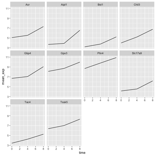
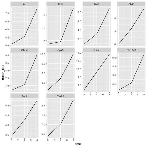
这里,各子图的 x 轴尺度保持一致,y 轴尺度也保持一致。你可以修改
scales 来改变这一默认行为,使每个子图的 y
轴采用各自的尺度:
R
ggplot(data = mean_exp_by_time,
       mapping = aes(x = time, y = mean_exp)) +
  geom_line() +
  facet_wrap(~ gene, scales = "free_y")
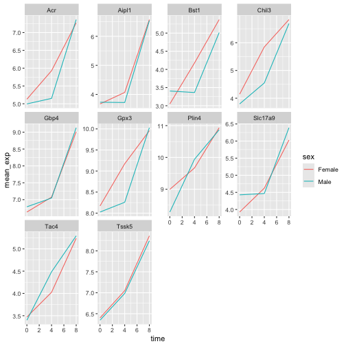
现在,我们想根据小鼠的性别来划分每个图表中的线条。为此,我们需要计算数据框中按
gene、time 和 sex
分组的平均表达量:
R
mean_exp_by_time_sex <- sub_rna |>
  group_by(gene, time, sex) |>
    summarize(mean_exp = mean(expression_log))
输出
`summarise()` has regrouped the output.
ℹ Summaries were computed grouped by gene, time, and sex.
ℹ Output is grouped by gene and time.
ℹ Use `summarise(.groups = "drop_last")` to silence this message.
ℹ Use `summarise(.by = c(gene, time, sex))` for per-operation grouping
  (`?dplyr::dplyr_by`) instead.
R
mean_exp_by_time_sex
输出
# A tibble: 60 × 4
# Groups:   gene, time [30]
   gene   time sex    mean_exp
   <chr> <int> <chr>     <dbl>
 1 Acr       0 Female     5.13
 2 Acr       0 Male       5.00
 3 Acr       4 Female     5.93
 4 Acr       4 Male       5.15
 5 Acr       8 Female     7.27
 6 Acr       8 Male       7.36
 7 Aipl1     0 Female     3.67
 8 Aipl1     0 Male       3.73
 9 Aipl1     4 Female     4.07
10 Aipl1     4 Male       3.72
# ℹ 50 more rows
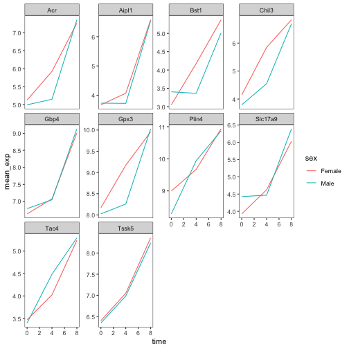
现在我们可以通过
color(在单个图表中)进一步按性别进行划分,从而创建分面图:
R
ggplot(data = mean_exp_by_time_sex,
       mapping = aes(x = time, y = mean_exp, color = sex)) +
  geom_line() +
  facet_wrap(~ gene, scales = "free_y")
通常,白色背景的图表在打印时更易于阅读。我们可以使用
theme_bw()
函数将背景设置为白色。此外,我们还可以移除网格:
R
ggplot(data = mean_exp_by_time_sex,
       mapping = aes(x = time, y = mean_exp, color = sex)) +
  geom_line() +
  facet_wrap(~ gene, scales = "free_y") +
  theme_bw() +
  theme(panel.grid = element_blank())
挑战
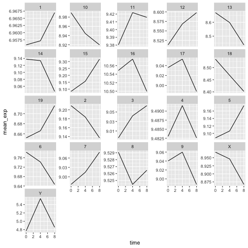
运用刚才学到的知识,绘制一张图表,展示每条染色体的平均表达量在感染过程中如何变化。
R
mean_exp_by_chromosome <- rna |>
  group_by(chromosome_name, time) |>
  summarize(mean_exp = mean(expression_log))
输出
`summarise()` has regrouped the output.
ℹ Summaries were computed grouped by chromosome_name and time.
ℹ Output is grouped by chromosome_name.
ℹ Use `summarise(.groups = "drop_last")` to silence this message.
ℹ Use `summarise(.by = c(chromosome_name, time))` for per-operation grouping
  (`?dplyr::dplyr_by`) instead.
R
ggplot(data = mean_exp_by_chromosome, mapping = aes(x = time,
                                y = mean_exp)) +
  geom_line() +
  facet_wrap(~ chromosome_name, scales = "free_y")
facet_wrap
会将子图自动排列成若干行和列,以便整齐地放在一页上。另一方面,facet_grid
允许你通过公式表示法显式指定子图的行列布局(rows ~ columns;其中
.
可用作占位符,表示该方向不进行分面,因而只有一行或一列)。
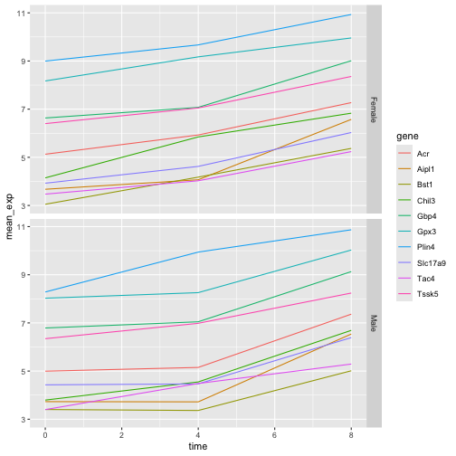
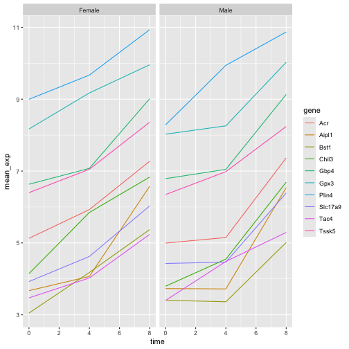
让我们修改之前的图表,以比较雄性和雌性的平均基因表达随时间的变化情况:
R
# One column, facet by rows
ggplot(data = mean_exp_by_time_sex,
       mapping = aes(x = time, y = mean_exp, color = gene)) +
  geom_line() +
  facet_grid(sex ~ .)
R
# One row, facet by column
ggplot(data = mean_exp_by_time_sex,
       mapping = aes(x = time, y = mean_exp, color = gene)) +
  geom_line() +
  facet_grid(. ~ sex)
ggplot2 主题
除了将图表背景改为白色的 theme_bw()
之外,ggplot2
还提供了其他几种主题,可用于快速更改可视化效果的外观。完整的主题列表可在
https://ggplot2.tidyverse.org/reference/ggtheme.html
中查看。theme_minimal() 和 theme_light()
非常受欢迎,而 theme_void()
则可作为创建自定义主题的起点。
ggthemes
包提供了多种选项(包括 Excel 2003 主题)。ggplot2
扩展网站 提供了一份扩展 ggplot2
功能的包列表,其中包括额外的主题。
自定义
让我们回到那张按基因分面的图:它展示了平均表达量随时间的变化,并按性别着色。
请查看 ggplot2
速查表,并思考如何改进该图表。
现在,我们可以将轴名称更改为比“time”和“mean_exp”更具信息量的名称,并为图表添加标题:
R
ggplot(data = mean_exp_by_time_sex,
       mapping = aes(x = time, y = mean_exp, color = sex)) +
  geom_line() +
  facet_wrap(~ gene, scales = "free_y") +
  theme_bw() +
  theme(panel.grid = element_blank()) +
  labs(title = "Mean gene expression by duration of the infection",
       x = "Duration of the infection (in days)",
       y = "Mean gene expression")
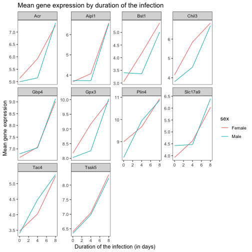
轴上的名称更具信息量,但可以通过增大字体大小来提高可读性:
R
ggplot(data = mean_exp_by_time_sex,
       mapping = aes(x = time, y = mean_exp, color = sex)) +
  geom_line() +
  facet_wrap(~ gene, scales = "free_y") +
  theme_bw() +
  theme(panel.grid = element_blank()) +
  labs(title = "Mean gene expression by duration of the infection",
       x = "Duration of the infection (in days)",
       y = "Mean gene expression")  +
  theme(text = element_text(size = 16))
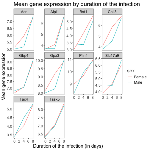
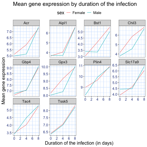
请注意,您也可以更改图表的字体。如果您使用的是 Windows,可能需要安装
extrafont
包。
我们还可以进一步自定义 x 轴和 y
轴文本的颜色、网格颜色等。例如,我们还可以通过将
legend.position 设置为 "top"
将图例移至顶部。
R
ggplot(data = mean_exp_by_time_sex,
       mapping = aes(x = time, y = mean_exp, color = sex)) +
  geom_line() +
  facet_wrap(~ gene, scales = "free_y") +
  theme_bw() +
  theme(panel.grid = element_blank()) +
  labs(title = "Mean gene expression by duration of the infection",
       x = "Duration of the infection (in days)",
       y = "Mean gene expression")  +
  theme(text = element_text(size = 16),
        axis.text.x = element_text(colour = "royalblue4", size = 12),
        axis.text.y = element_text(colour = "royalblue4", size = 12),
        panel.grid = element_line(colour="lightsteelblue1"),
        legend.position = "top")
如果你更喜欢自己做出的修改而非默认主题,可以将它们保存为对象,以便轻松应用于你可能创建的其他图表。以下是一个使用我们之前创建的直方图的示例。
R
blue_theme <- theme(axis.text.x = element_text(colour = "royalblue4",
                                               size = 12),
                    axis.text.y = element_text(colour = "royalblue4",
                                               size = 12),
                    text = element_text(size = 16),
                    panel.grid = element_line(colour="lightsteelblue1"))

ggplot(rna, aes(x = expression_log)) +
  geom_histogram(bins = 20) +
    blue_theme
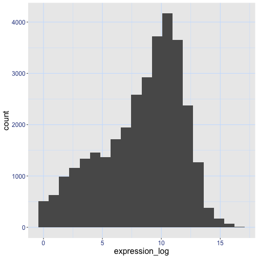
挑战
有了所有这些信息,请再花五分钟时间,要么改进本练习中生成的其中一张图表,要么创建一张精美的图表。可以参考
RStudio 的 ggplot2
速查表 寻找灵感。以下是一些建议:
- 看看能否更改线条的粗细。
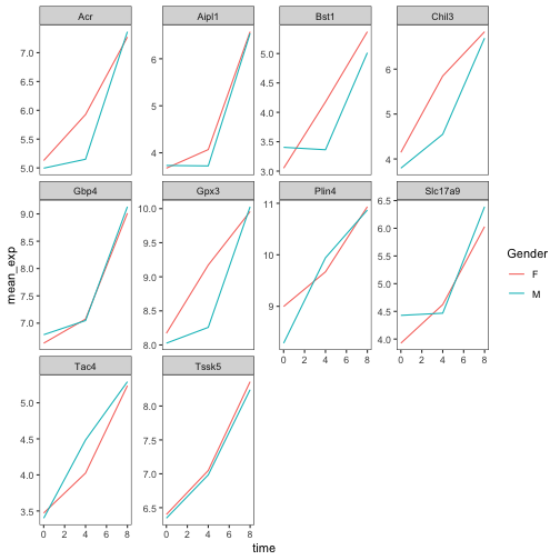
- 你能找到修改图例名称的方法吗?那么其标签呢?(提示:寻找以
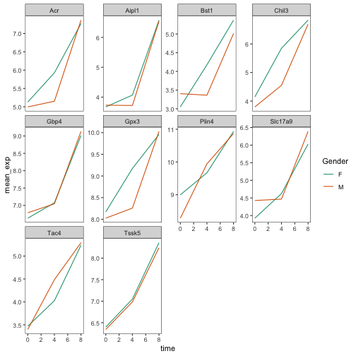
scale_开头的 ggplot 函数) - 尝试使用不同的配色方案,或手动指定线条的颜色(参见 https://www.cookbook-r.com/Graphs/Colors_(ggplot2)/)。
例如,基于这张图:
R
ggplot(data = mean_exp_by_time_sex,
       mapping = aes(x = time, y = mean_exp, color = sex)) +
  geom_line() +
  facet_wrap(~ gene, scales = "free_y") +
  theme_bw() +
  theme(panel.grid = element_blank())
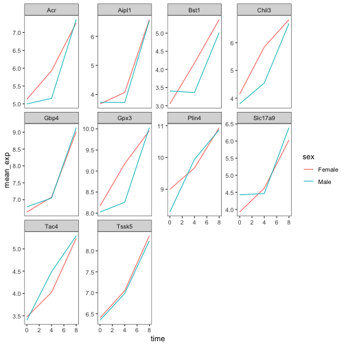
我们可以通过以下方式对其进行自定义:
R
# change the thickness of the lines
ggplot(data = mean_exp_by_time_sex,
       mapping = aes(x = time, y = mean_exp, color = sex)) +
  geom_line(size=1.5) +
  facet_wrap(~ gene, scales = "free_y") +
  theme_bw() +
  theme(panel.grid = element_blank())
警告
Warning: Using `size` aesthetic for lines was deprecated in ggplot2 3.4.0.
ℹ Please use `linewidth` instead.
This warning is displayed once per session.
Call `lifecycle::last_lifecycle_warnings()` to see where this warning was
generated.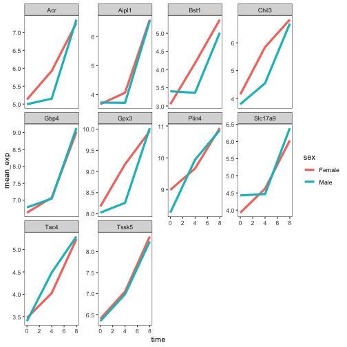
R
# change the name of the legend and the labels
ggplot(data = mean_exp_by_time_sex,
       mapping = aes(x = time, y = mean_exp, color = sex)) +
  geom_line() +
  facet_wrap(~ gene, scales = "free_y") +
  theme_bw() +
  theme(panel.grid = element_blank()) +
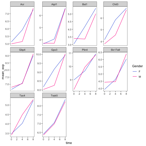
  scale_color_discrete(name = "Gender", labels = c("F", "M"))
R
# using a different color palette
ggplot(data = mean_exp_by_time_sex,
       mapping = aes(x = time, y = mean_exp, color = sex)) +
  geom_line() +
  facet_wrap(~ gene, scales = "free_y") +
  theme_bw() +
  theme(panel.grid = element_blank()) +
  scale_color_brewer(name = "Gender", labels = c("F", "M"), palette = "Dark2")
R
# manually specifying the colors
ggplot(data = mean_exp_by_time_sex,
       mapping = aes(x = time, y = mean_exp, color = sex)) +
  geom_line() +
  facet_wrap(~ gene, scales = "free_y") +
  theme_bw() +
  theme(panel.grid = element_blank()) +
  scale_color_manual(name = "Gender",  labels = c("F", "M"),
                     values = c("royalblue", "deeppink"))
合成图表
Faceting 是将一个图表拆分为多个子图的绝佳工具,但有时你可能希望生成一个包含多个独立图表的单一图表,即基于不同变量甚至不同数据框的图表。
让我们先创建这两个想要并排显示的图表:
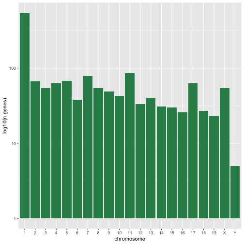
第一张图统计每条染色体上不同基因的数量。我们首先需要重新排列
chromosome_name
的因子水平,并对每条染色体上的基因去重。此外,我们还将 y 轴改为 log10
尺度,以提高可读性。
R
rna$chromosome_name <- factor(rna$chromosome_name,
                               levels = c(1:19,"X","Y"))

count_gene_chromosome <- rna |>
  select(chromosome_name, gene) |>
  distinct() |> ggplot() +
  geom_bar(aes(x = chromosome_name), fill = "seagreen",
           position = "dodge", stat = "count") +
  labs(y = "log10(n genes)", x = "chromosome") +
  scale_y_log10()

count_gene_chromosome
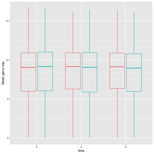
下面,我们还通过将 legend.position 设置为
"none" 来完全移除图例。
R
exp_boxplot_sex <- ggplot(rna, aes(y=expression_log, x = as.factor(time),
                 color=sex)) +
   geom_boxplot(alpha = 0) +
  labs(y = "Mean gene exp",
       x = "time") + theme(legend.position = "none")

exp_boxplot_sex
patchwork
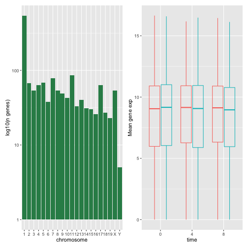
包提供了一种简洁的方法,利用 +
来组合图表(通常为并排排列)。具体而言,|
将图表并排排列,而 / 则将它们上下排列。
R
install.packages("patchwork")
R
library("patchwork")
count_gene_chromosome + exp_boxplot_sex
R
## or count_gene_chromosome | exp_boxplot_sex
R
count_gene_chromosome / exp_boxplot_sex
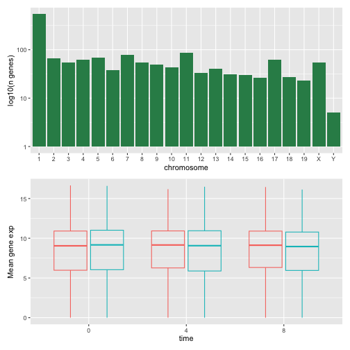
我们可以进一步使用 plot_layout
来控制最终合成图的布局,从而创建更复杂的布局:
R
count_gene_chromosome + exp_boxplot_sex + plot_layout(ncol = 1)
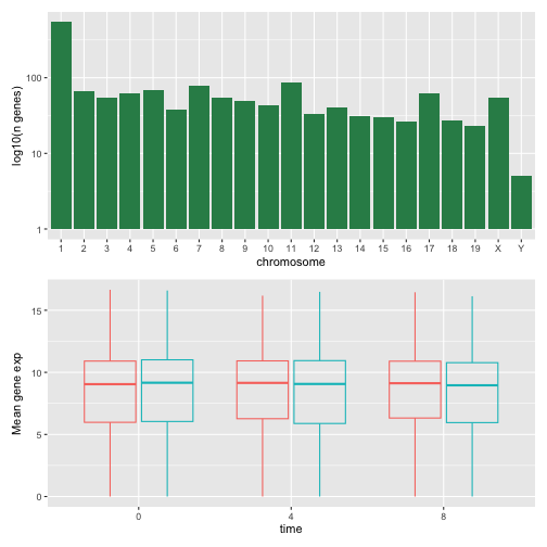
R
count_gene_chromosome +
 (count_gene_chromosome + exp_boxplot_sex) +
 exp_boxplot_sex +
 plot_layout(ncol = 1)
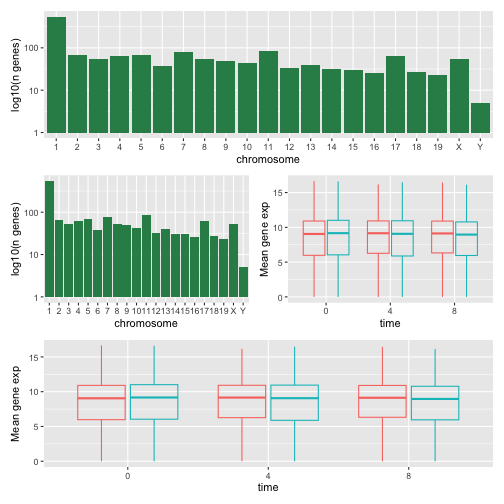
最后一个图表也可以使用 | 和 /
组件来创建:
R
count_gene_chromosome /
 (count_gene_chromosome | exp_boxplot_sex) /
 exp_boxplot_sex
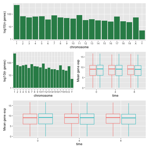
欲了解更多关于 patchwork 的信息,请访问其 网页 或观看此 视频。
另一种选择是 gridExtra 包,它允许使用
grid.arrange() 将独立的 ggplot 合并为单个图表:
R
install.packages("gridExtra")
R
library("gridExtra")
grid.arrange(count_gene_chromosome, exp_boxplot_sex, ncol = 2)
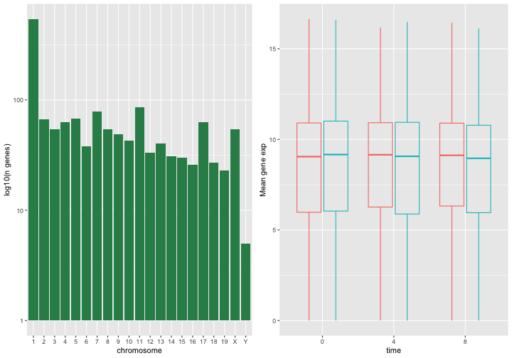
除了用于简单布局的 ncol 和 nrow
参数外,还提供了用于构建更复杂布局的工具。
导出图表
创建图表后,您可以将其保存为您喜欢的格式的文件。RStudio 中 Plot 窗格的“Export”选项卡会以低分辨率保存图表,这不被许多期刊接受,且在海报展示时无法良好地缩放。
相反,请使用 ggsave()
函数,通过调整相应的参数(width、height 和
dpi),即可轻松更改图表的尺寸和分辨率。
请确保您的工作目录中包含 fig_output/ 文件夹。
R
my_plot <- ggplot(data = mean_exp_by_time_sex,
       mapping = aes(x = time, y = mean_exp, color = sex)) +
  geom_line() +
  facet_wrap(~ gene, scales = "free_y") +
  labs(title = "Mean gene expression by duration of the infection",
         x = "Duration of the infection (in days)",
         y = "Mean gene expression") +
  guides(color=guide_legend(title="Gender")) +
  theme_bw() +
  theme(axis.text.x = element_text(colour = "royalblue4", size = 12),
        axis.text.y = element_text(colour = "royalblue4", size = 12),
        text = element_text(size = 16),
        panel.grid = element_line(colour="lightsteelblue1"),
        legend.position = "top")
ggsave("fig_output/mean_exp_by_time_sex.png", my_plot, width = 15,
       height = 10)

# This also works for grid.arrange() plots
combo_plot <- grid.arrange(count_gene_chromosome, exp_boxplot_sex,
                           ncol = 2, widths = c(4, 6))
ggsave("fig_output/combo_plot_chromosome_sex.png", combo_plot,
       width = 10, dpi = 300)
注:参数 width 和 height
还会决定保存后图表中的字体大小。
其他可视化包
ggplot2 是一个非常强大的包,与我们的 整洁数据
和 整洁工具 流水线非常契合。R
中还有其他不容忽视的可视化包。
基础图形库
R 自带的默认图形系统(通常称为 base R
graphics)简单且快速。它基于
画家或画布模型,其中不同的输出直接叠加在一起(见下图)。这与
ggplot2(以及下文介绍的
lattice)有着本质的区别,后者返回专门的对象,可在屏幕或文件中渲染,甚至可以更新。
R
par(mfrow = c(1, 3))
plot(1:20, main = "First layer, produced with plot(1:20)")

plot(1:20, main = "A horizontal red line, added with abline(h = 10)")
abline(h = 10, col = "red")

plot(1:20, main = "A rectangle, added with rect(5, 5, 15, 15)")
abline(h = 10, col = "red")
rect(5, 5, 15, 15, lwd = 3)
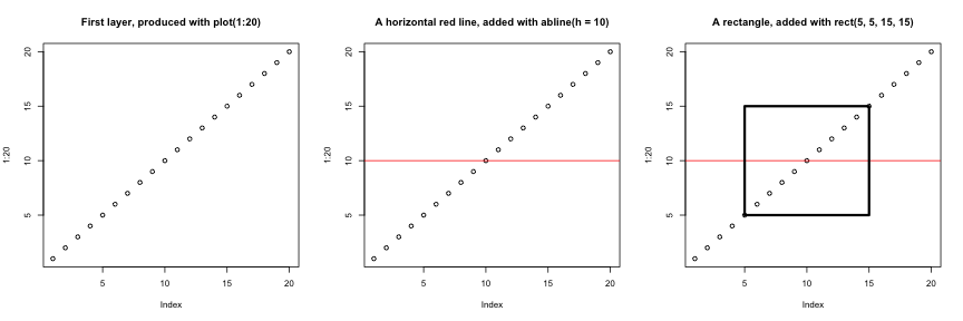
另一个主要区别在于,基础图形库的绘图函数会尝试根据输入类型采取正确的处理方式,即它们会根据输入的类别来调整行为。这与
ggplot2
的做法又大相径庭,后者仅接受数据框作为输入,且要求绘图必须逐步构建。
R
par(mfrow = c(2, 2))
boxplot(rnorm(100),
        main = "Boxplot of rnorm(100)")
boxplot(matrix(rnorm(100), ncol = 10),
        main = "Boxplot of matrix(rnorm(100), ncol = 10)")
hist(rnorm(100))
hist(matrix(rnorm(100), ncol = 10))
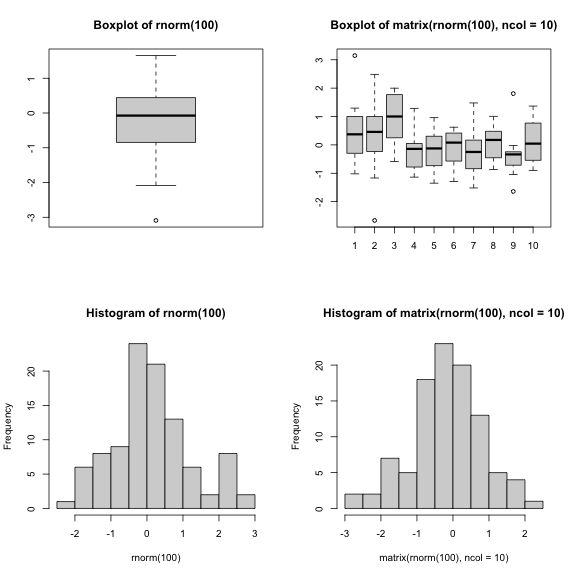
基础图形库的开箱即用方式对于简单的标准图表非常高效,只需一行代码和单个函数(如
plot、hist 或 boxplot
等)即可快速生成。然而,默认设置并不总是最理想,且图表的调优——尤其是当图表变得复杂时(例如为了生成分面)——可能会变得冗长且繁琐。
lattice 包
lattice 包与 ggplot2
类似,均以数据框作为输入,返回图形对象并支持分面。然而,lattice
并非基于图形语法,且其接口更为复杂。
lattice 包的良好参考资料是 Deepayan (2008).
- R 中的可视化