所有图片
使用电子表格组织数据
图 1
第 1 张图片,共 1 张:‘SCreenshot of a spreadsheet and a README.txt file.’
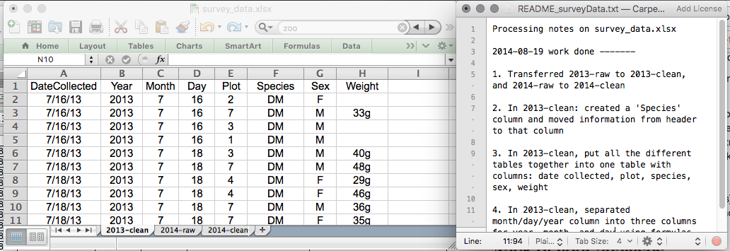
图 2
第 1 张图片,共 1 张:‘A table showing the blood and rhesus types encoded together in one column.’
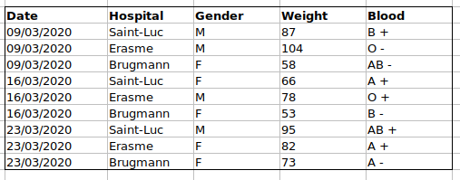
图 3
第 1 张图片,共 1 张:‘A table showing the blood and rhesus types encoded together in different columns.’
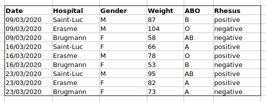
图 4
第 1 张图片,共 1 张:‘A sheet with many subtable.’
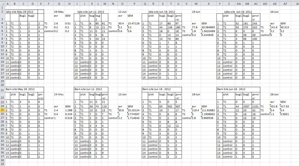
图 5
第 1 张图片,共 1 张:‘A table extracted from a paper showing commonly used null values.’
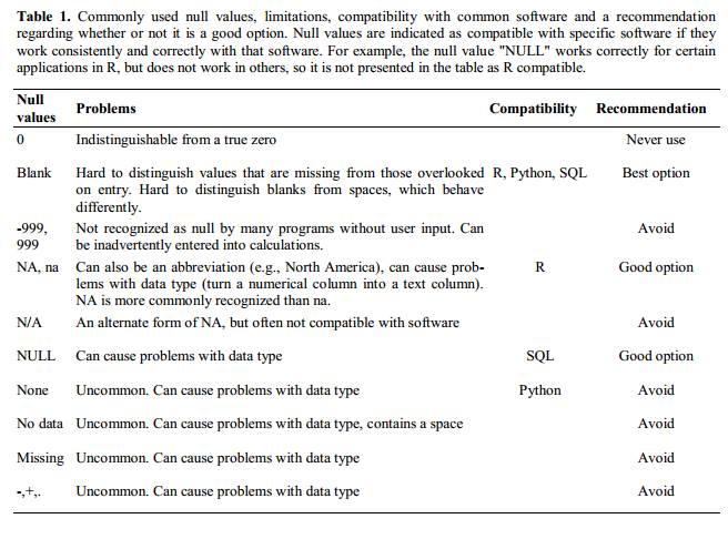
图 6
第 1 张图片,共 1 张:‘A table showing several cells highlighted in yellow used to encode sample contamination.’
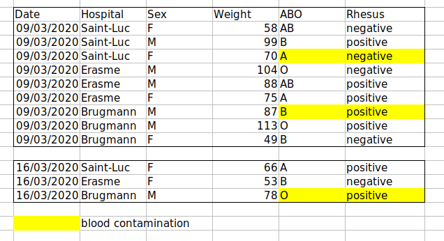
图 7
第 1 张图片,共 1 张:‘Same table as above with a new variable encoding contambination.’
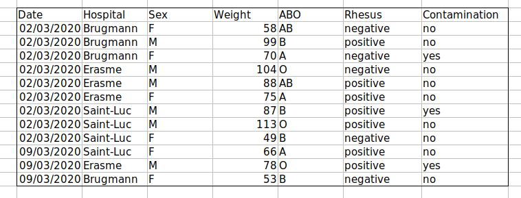
图 8
第 1 张图片,共 1 张:‘Excel menu to export data in a csv format on MacOS ’
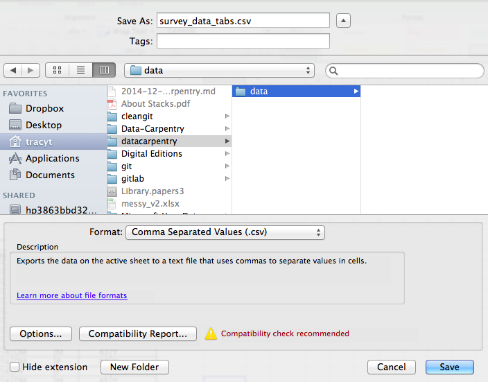
图 9
第 1 张图片,共 1 张:‘A table illustrating ill-imported data that contained a comma in a cell. That cell has been split in two cells.’
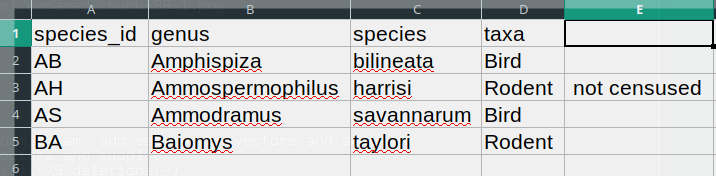
图 10
第 1 张图片,共 1 张:‘The tidy data analysis circle, iterating over data transformation, visualisation and modelling.’
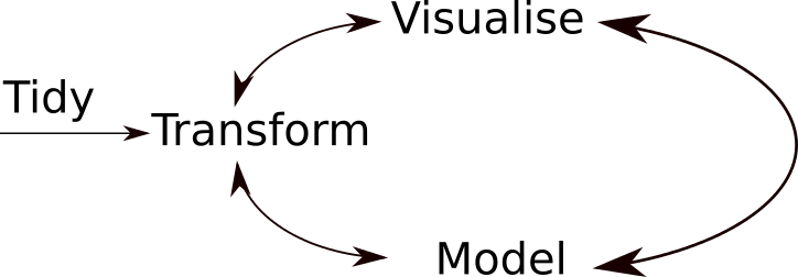
R 和 RStudio
图 1
第 1 张图片,共 1 张:‘Two graphs showing the exponential increase of the number of CRAN packages from 2000 to 2018. The figure on the right shows linear trend for the log of number of packages.’
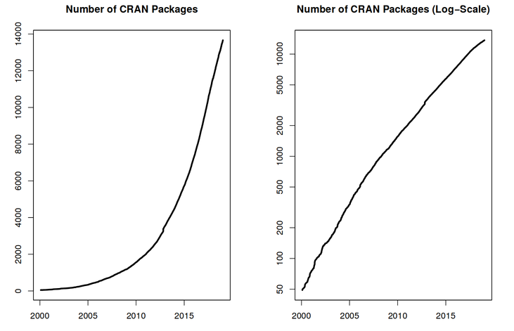
图 2
第 1 张图片,共 1 张:‘Screenshot of the RStudio interface showing the typical four panel setup.’
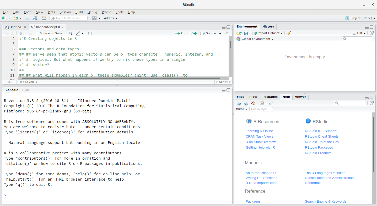
图 3
第 1 张图片,共 1 张:‘Screenshot of the RStudio General Options panel.’
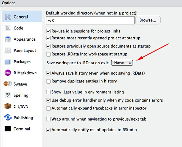
图 4
第 1 张图片,共 1 张:‘Screenshot of the RStudio Code Options panel.’
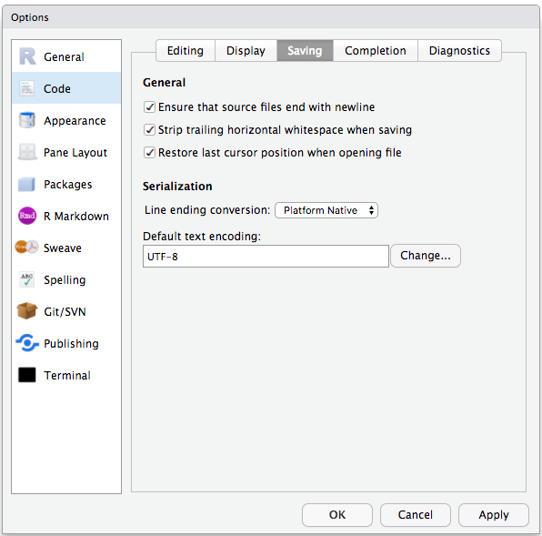
图 5
第 1 张图片,共 1 张:‘Flow diagram showing the structure of the working directory and various directory of a typical RStuio project.’
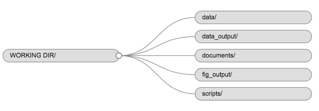
图 6
第 1 张图片,共 1 张:‘Screenshot of RStudio's Files panel.’
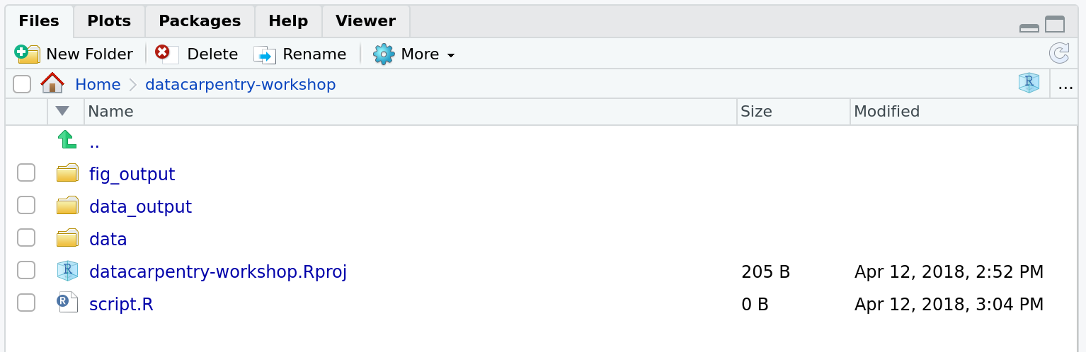
图 7
第 1 张图片,共 1 张:‘Figure form Nobel et al. (2009) showing a complex bioinformatics project structure.’
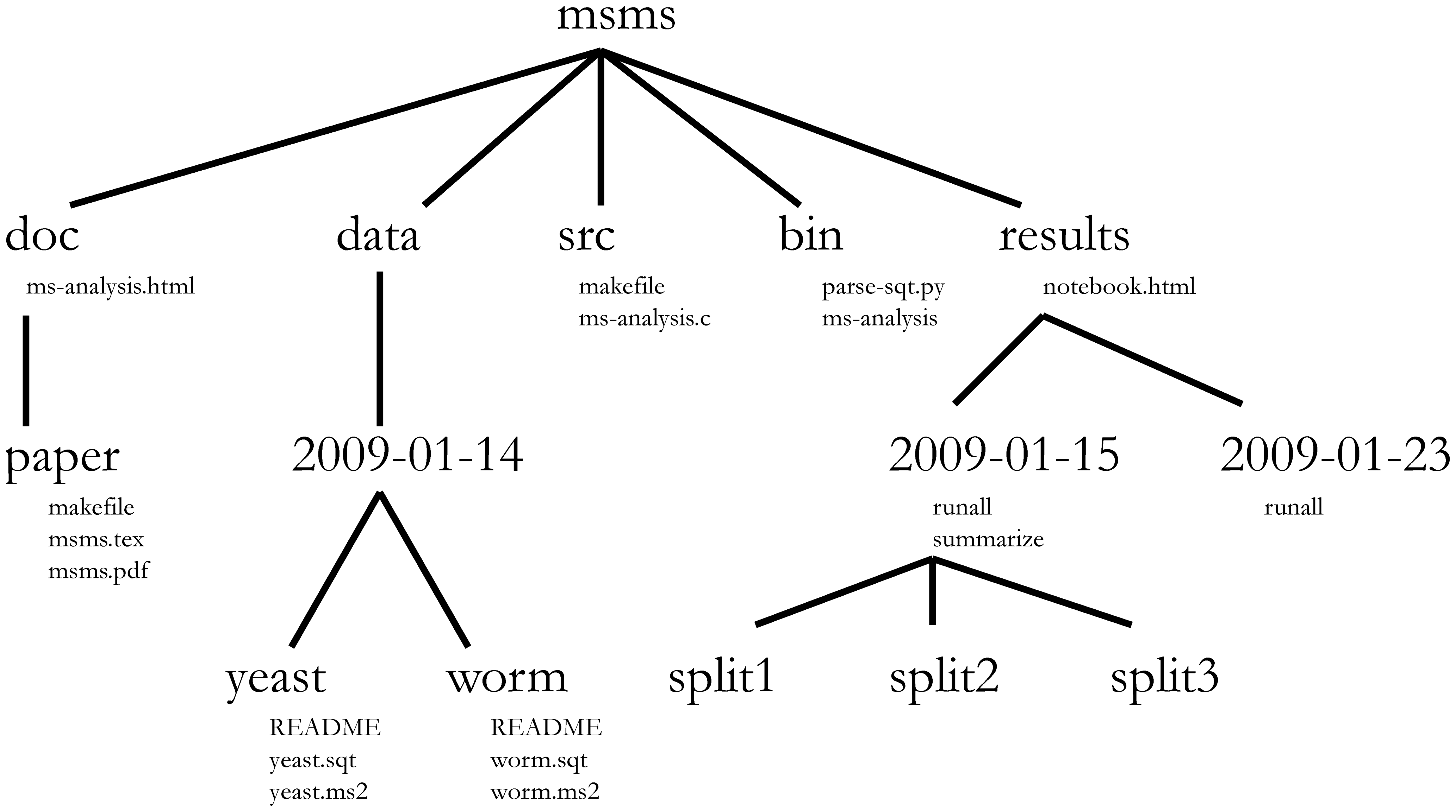
图 8
第 1 张图片,共 1 张:‘Fake book cover showing a kitten with title 'Changing Stuff and Seeing What Happens.'’
图 9
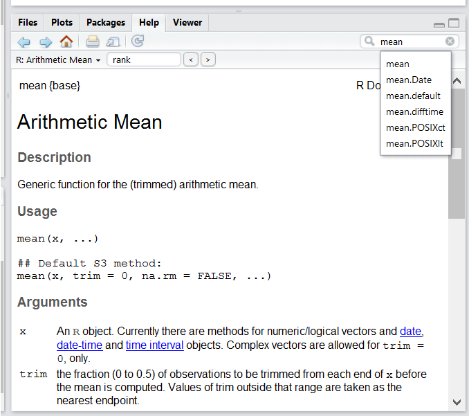
第 1 张图片,共 1 张:‘Screenshot of RStudio's Help panel.’
R 入门
图 1
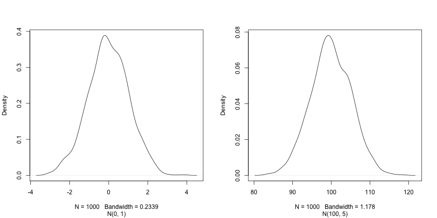
第 1 张图片,共 1 张:‘Two figures illustraing normal distributonis N(0,1) and N(100,5).’
从数据开始
图 1
第 1 张图片,共 1 张:‘Schematic representation of a tablular structure with different colours representing different columns and variables types.’
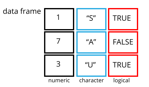
图 2
第 1 张图片,共 1 张:‘Barplot showing the number of 'male' and 'female' occurrences.’
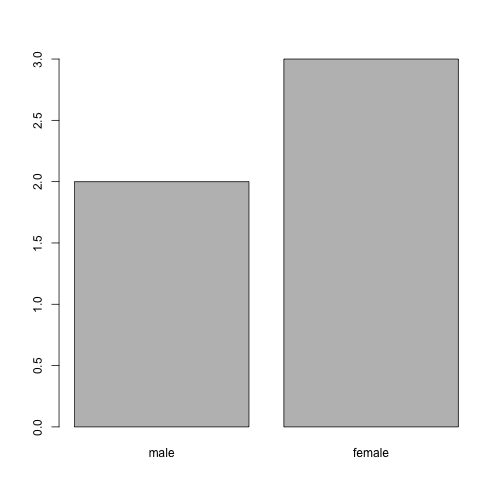
图 3
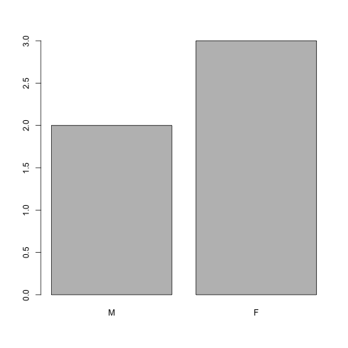
第 1 张图片,共 1 张:‘Barplot showing the number of 'M' and 'F' occurrences.’
使用 dplyr 处理和分析数据
图 1
第 1 张图片,共 1 张:‘Figure showing the long table format on the left and wide table format on the right and arrows illustrating how the values in the 'sample' column on the left have become column names on the right and how the values in the 'expression' column on the left have become values on the the right. Below is the call to 'pivot_wider()' with annotations pointing to the 'sample' and 'expression' function arguments.’
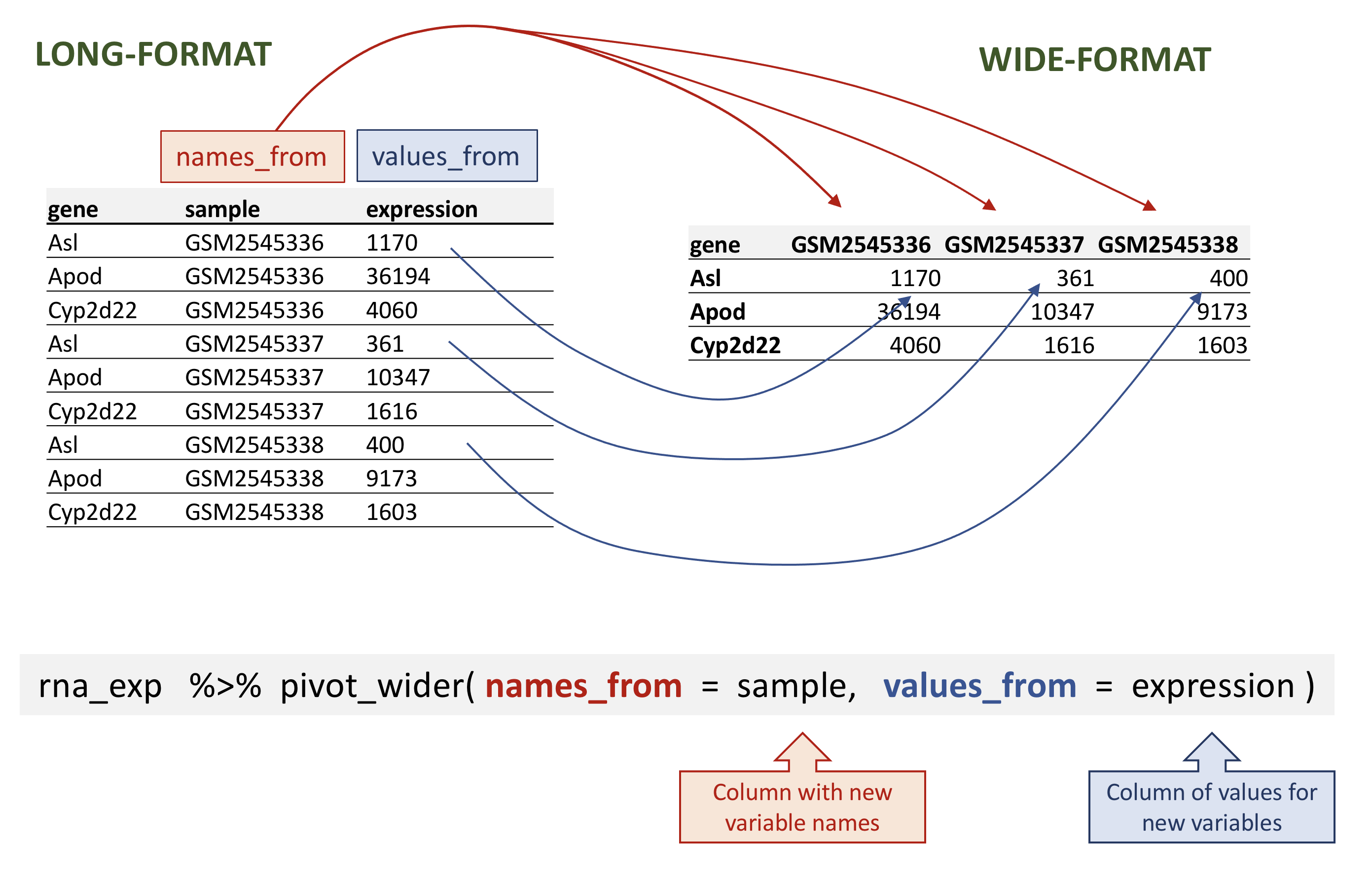
rna data.
图 2
第 1 张图片,共 1 张:‘Figure showing the long table format on the left and wide table format on the right and arrows illustrating how the column names on the left have become a new column 'sample' on the left and the values in the wide table on the right have become a new column 'expression' on the left. Below is the call to 'pivot_wider()' with annotations pointing to the 'sample', 'expression' and the '-gene' arguments.’
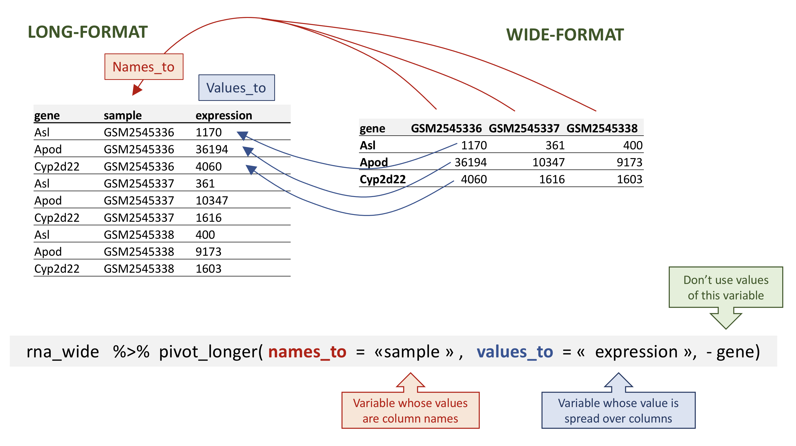
rna data.
图 3
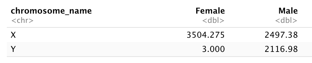
第 1 张图片,共 1 张:‘A two by two table with X and Y row names and Female and Male column names showing the total counts for each X/Y and Female/Male combination. The Y/Female combinations shows 3 counts, while all other counts are above 2000 counts.’
数据可视化
图 1
第 1 张图片,共 1 张:‘Default histogram produced by ggplot() and geom_histogram() for the expression data.’
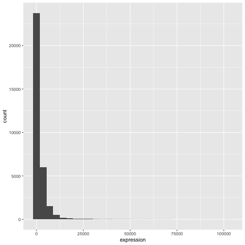
图 2
第 1 张图片,共 1 张:‘Histograms produced by ggplot() and geom_histogram() for the expression data with bin set of 15 (top) and binwith set to 2000 (bottom).’
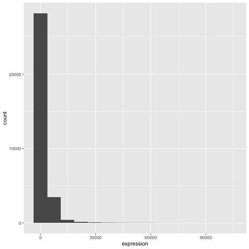
图 3
第 1 张图片,共 1 张:‘Histograms produced by ggplot() and geom_histogram() for the expression data with bin set of 15 (top) and binwith set to 2000 (bottom).’
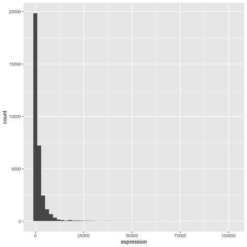
图 4
第 1 张图片,共 1 张:‘Histogram produced by ggplot() and geom_histogram() for the pre-computed log of expression.’
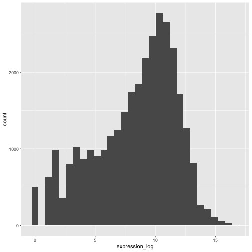
图 5
第 1 张图片,共 1 张:‘Histogram produced by ggplot(), geom_histogram() and scale_x_log10() for the log of expression.’
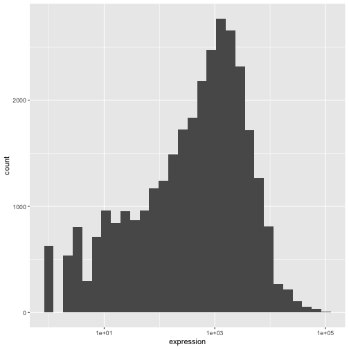
图 6
第 1 张图片,共 1 张:‘Scatter plot produced by ggplot() and geom_point() comparing the log-foldchanges computed above. All dots are black.’
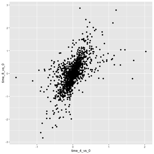
图 7
第 1 张图片,共 1 张:‘Scatter plot produced by ggplot() and geom_point() comparing the log-foldchanges computed above. All dots are semi-transparent black.’
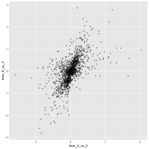
图 8
第 1 张图片,共 1 张:‘Scatter plot produced by ggplot() and geom_point() comparing the log-foldchanges computed above. All dots are semi-transparent blue.’
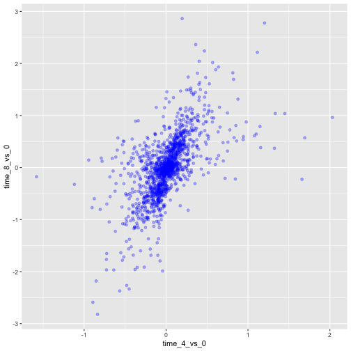
图 9
第 1 张图片,共 1 张:‘Scatter plot produced by ggplot() and geom_point() comparing the log-foldchanges computed above. Dots are colour-coded based on the gene's biotype.’
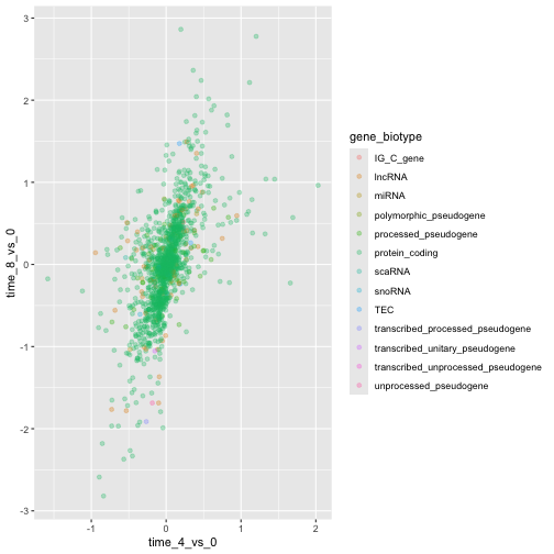
图 10
第 1 张图片,共 1 张:‘Scatter plot produced by ggplot() and geom_point() comparing the log-foldchanges computed above. Dots are colour-coded based on the gene's biotype.’
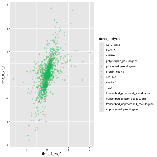
图 11
第 1 张图片,共 1 张:‘Scatter plot produced by ggplot() and geom_point() comparing the log-foldchanges computed above. Dots are colour-coded based on the gene's biotype. A black line of slope 1 crossing the origin was added by geom_abline().’
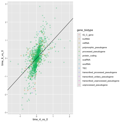
图 12
第 1 张图片,共 1 张:‘Scatter plot produced by ggplot() and geom_point() comparing the log-foldchanges computed above. Dots are colour-coded based on the gene's biotype. A black line of slope 1 crossing the origin was added by geom_abline().’
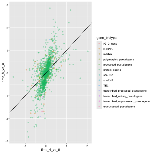
图 13
第 1 张图片,共 1 张:‘Scatter plot produced by ggplot() and geom_hexbin() comparing the log-foldchanges computed above shows hexagons coloured based on the underlying dot density. A black line of slope 1 crossing the origin was added by geom_abline().’
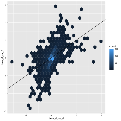
图 14
第 1 张图片,共 1 张:‘Figures showing a stretch of overlapping points indicating the log of expression + 1 for each sample. The points are coloured with different shades of blue for samples collected at different time points.’
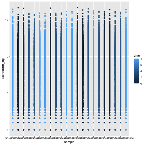
图 15
第 1 张图片,共 1 张:‘Boxplot showing the distribution of log expression + 1 values for each sample, as produced by geom_boxlpot(). Each boxplot is filled with white colour.’
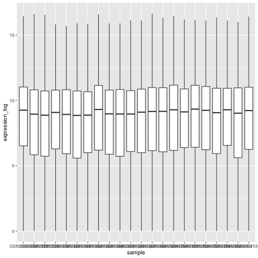
图 16
第 1 张图片,共 1 张:‘Boxplot and dots showing the distribution of log expression + 1 values for each sample, as produced by geom_boxlpot(). Each boxplot is transparent and the jittered dots are semi-transparent tomato-coloured and behind the boxpots.’
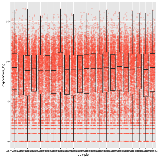
图 17
第 1 张图片,共 1 张:‘Boxplot and dots showing the distribution of log expression + 1 values for each sample, as produced by geom_boxlpot(). Each boxplot is transparent and the jittered dots are semi-transparent tomato-coloured. This time, the boxplots are behind the dots.’
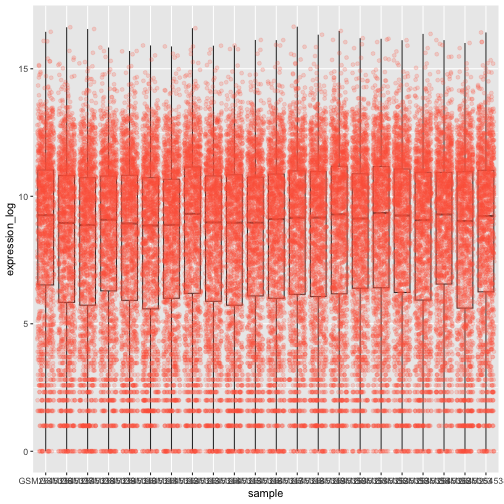
图 18
第 1 张图片,共 1 张:‘Boxplot and dots showing the distribution of log expression + 1 values for each sample, as produced by geom_boxlpot(). Each boxplot is transparent and the jittered dots are semi-transparent tomato-coloured. The sample labels are displayed vertically and readable.’
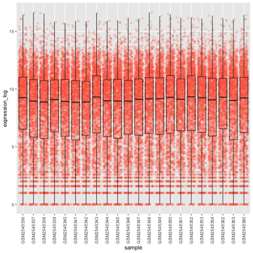
图 19
第 1 张图片,共 1 张:‘Boxplot and dots showing the distribution of log expression + 1 values for each sample, as produced by geom_boxlpot(). On the first figure, each boxplot is transparent and the jittered dots are semi-transparent and coloured in different shares of blue. On the second figures, each boxplot is transparent and the jittered dots are semi-transparent and coloured red, green and blue.’
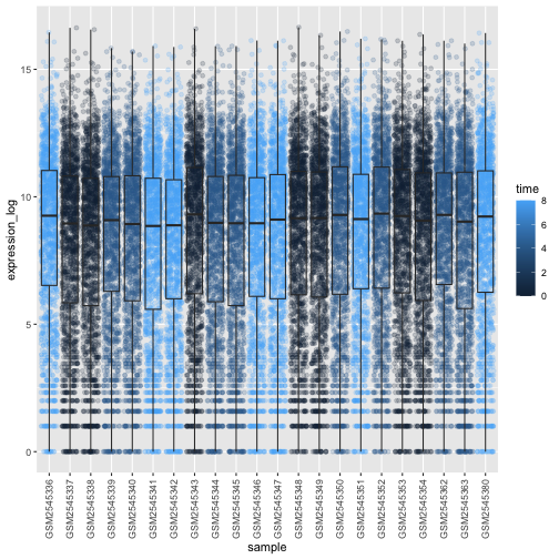
图 20
第 1 张图片,共 1 张:‘Boxplot and dots showing the distribution of log expression + 1 values for each sample, as produced by geom_boxlpot(). On the first figure, each boxplot is transparent and the jittered dots are semi-transparent and coloured in different shares of blue. On the second figures, each boxplot is transparent and the jittered dots are semi-transparent and coloured red, green and blue.’
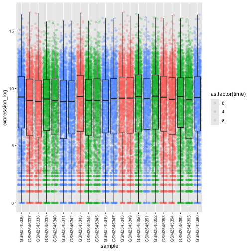
图 21
第 1 张图片,共 1 张:‘Violin plot showing the distribution of log expression + 1 values for each sample, as produced by geom_violin(). Each boxplot is transparent and the jittered dots are semi-transparent and coloured red, green and blue.’
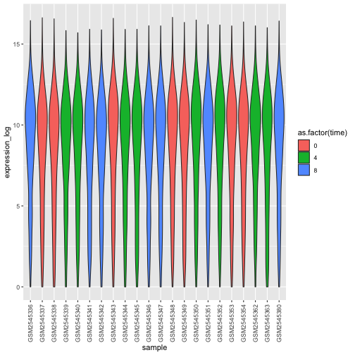
图 22
第 1 张图片,共 1 张:‘Violin plot showing the distribution of log expression + 1 values for each sample, as produced by geom_violon(). Each violin plot is coloured in red or blue depending on the sex variable.’
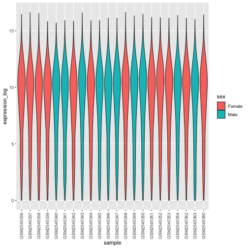
图 23
第 1 张图片,共 1 张:‘Line plot, as produced by geom_line(), but the lines are clearly not show what we expect.’
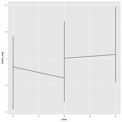
图 24
第 1 张图片,共 1 张:‘Line plot, as produced by geom_line(), with 10 lines showing increasing expression values over time.’
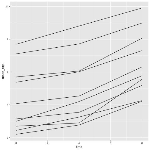
图 25
第 1 张图片,共 1 张:‘Line plot, as produced by geom_line(), with 10 colour-coded lines showing increasing expression values over time.’
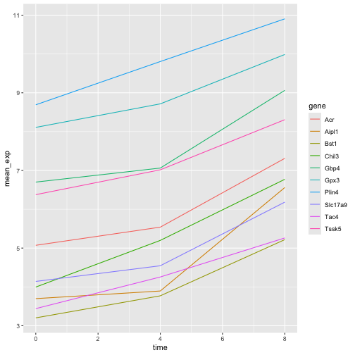
图 26
第 1 张图片,共 1 张:‘Line plot, as produced by geom_line(), with 10 sub-plots/facets, each showing one line with increasing expression values over time. All y-scales are identical.’
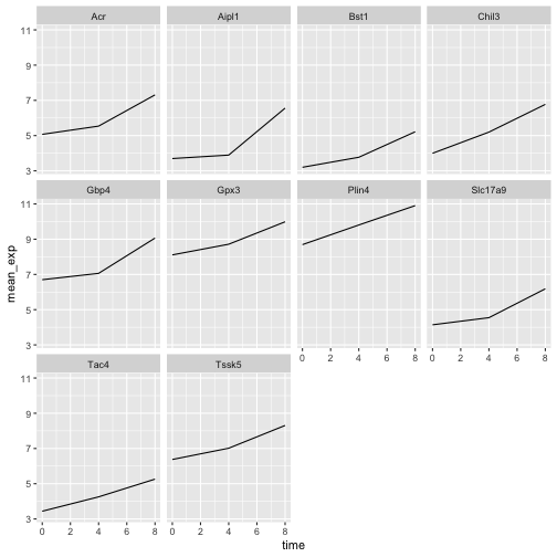
图 27
第 1 张图片,共 1 张:‘Line plot, as produced by geom_line(), with 10 sub-plots/facets, each showing one line with increasing expression values over time. y-scales are now adapted to the expression range for each facet/gene.’
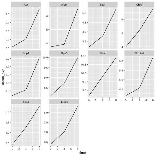
图 28
第 1 张图片,共 1 张:‘Line plot, as produced by geom_line(), with 10 sub-plots/facets, each showing two coloured lines (red for Female and blue for Make) with increasing expression values over time.’
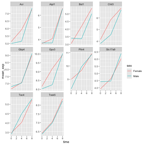
图 29
第 1 张图片,共 1 张:‘Line plot, as produced by geom_line(), with 10 sub-plots/facets, each showing two coloured lines (red for Female and blue for Make) with increasing expression values over time. The figure background is now white.’
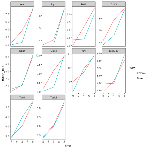
图 30
第 1 张图片,共 1 张:‘Line plot, as produced by geom_line(), with 21 sub-plots/facets, each showing one line with expression values over time for each chromosome.’
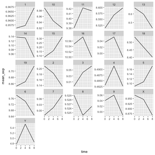
图 31
第 1 张图片,共 1 张:‘Two line plots above each other, each showing 10 lines coloured by gene. The top facet shows the expression values for Female sample, the bottom one for Male samples.’
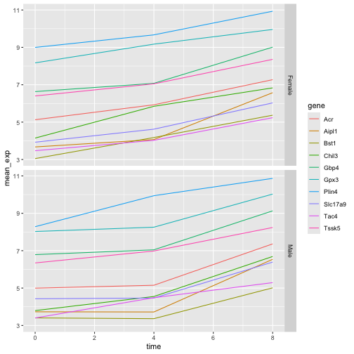
图 32
第 1 张图片,共 1 张:‘Two line plots next to each other, each showing 10 lines coloured by gene. The left facet shows the expression values for Female sample, the right one for Male samples.’
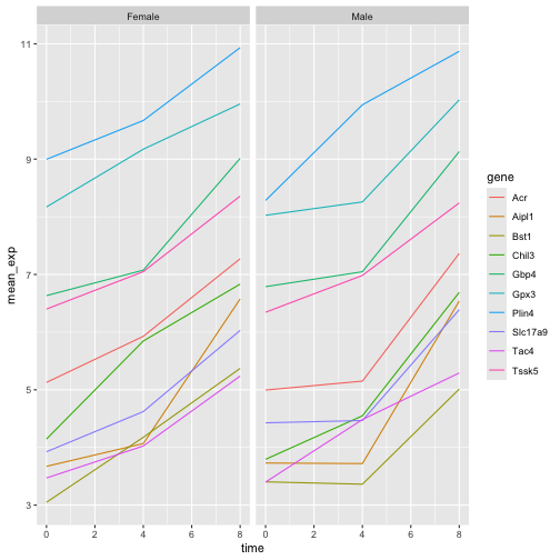
图 33
第 1 张图片,共 1 张:‘Line plot with white background and custom title and axis legends.’
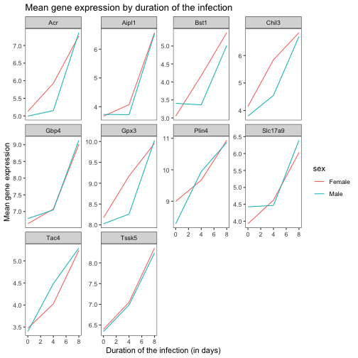
图 34
第 1 张图片,共 1 张:‘Line plot with white background and larger custom title and axis legends.’
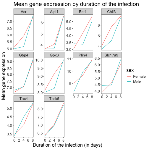
图 35
第 1 张图片,共 1 张:‘Line plot with white background and larger custom title and axis legends and blue grid.’
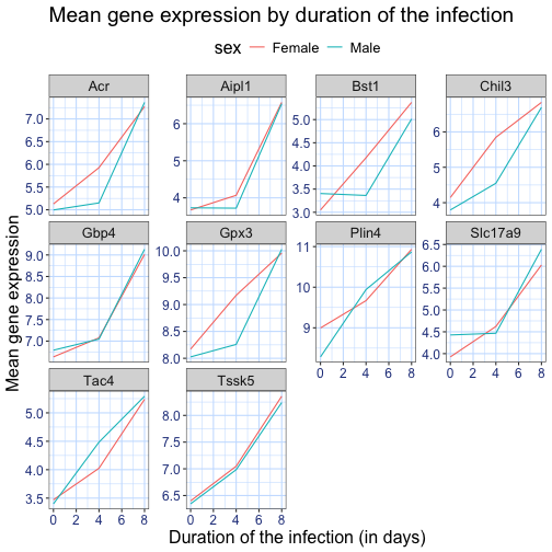
图 36
第 1 张图片,共 1 张:‘Custrom 'blue_theme() showing a blue grid and blue axis legends.’
图 37
第 1 张图片,共 1 张:‘Plain facetted line plot, as produced by theme_bw() and a blank grid above.’
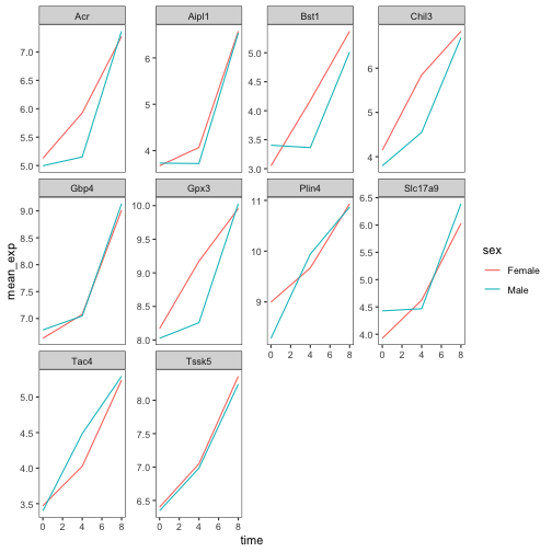
图 38
第 1 张图片,共 1 张:‘Plain facetted line plot, as produced by theme_bw() and a blank grid with wide lines.’
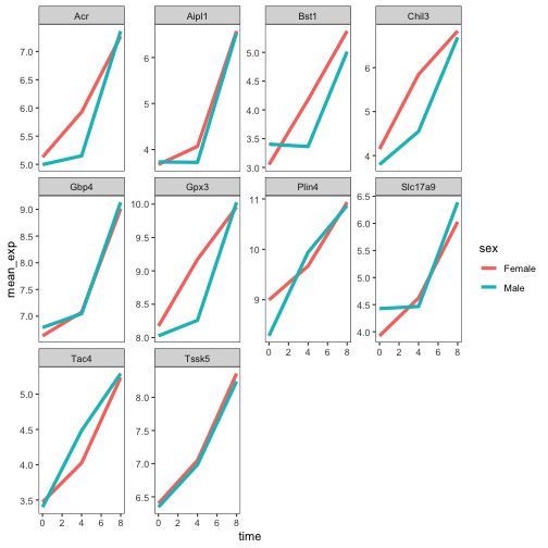
图 39
第 1 张图片,共 1 张:‘Plain facetted line plot, as produced by theme_bw() and a blank grid with renamed colour labels.’
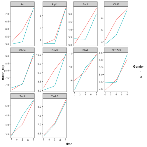
图 40
第 1 张图片,共 1 张:‘Plain facetted line plot, as produced by theme_bw() and a blank grid with a different color palette and renamed colour labels.’
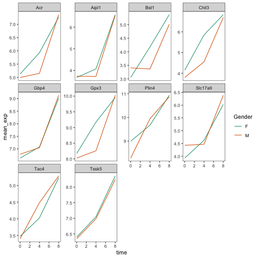
图 41
第 1 张图片,共 1 张:‘Plain facetted line plot, as produced by theme_bw() and a blank grid with a manually-set colors and renamed colour labels..’
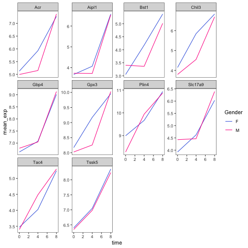
图 42
第 1 张图片,共 1 张:‘A simple histogram with greed bars showing the log10 number of genes per chromosome.’
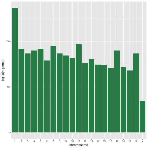
图 43
第 1 张图片,共 1 张:‘Transparently-filled red and blue boxplots for Female and Male expression values for different time points.’
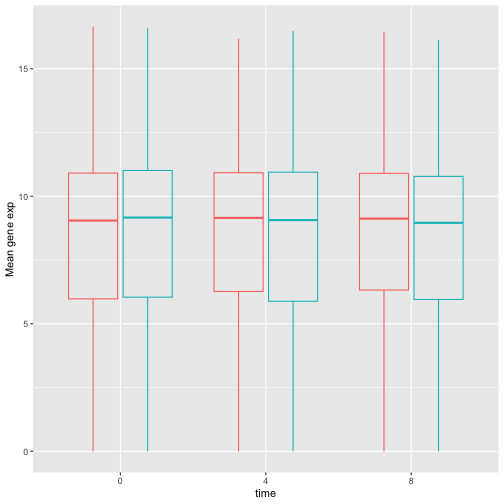
图 44
第 1 张图片,共 1 张:‘A composed figure show the histogram (left) and boxplots (right) next to each other.’
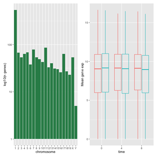
图 45
第 1 张图片,共 1 张:‘A composed figure show the histogram (top) and boxplots (bottom) on top or each other.’
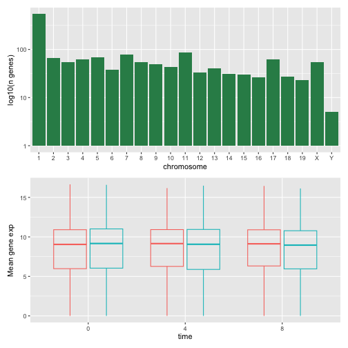
图 46
第 1 张图片,共 1 张:‘A composed figure show the histogram (top) and boxplots (bottom) on top or each other.’
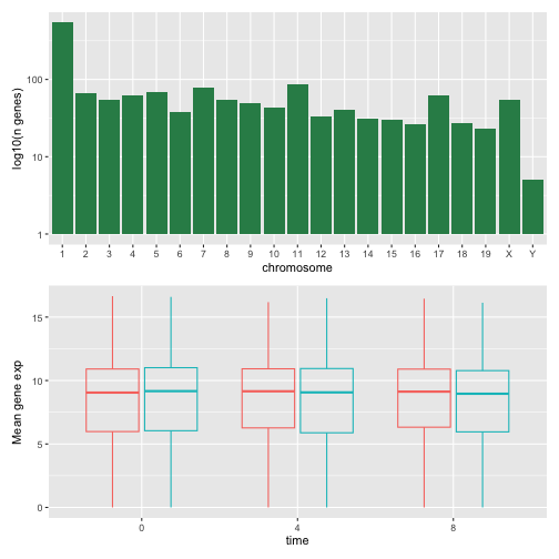
图 47
第 1 张图片,共 1 张:‘A figure composed of 4 plots with on top the histogram, in the middle the histogram and the boxpot, side-by-side, and at the bottom, the boxplot.’
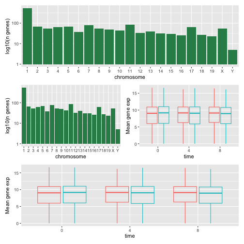
图 48
第 1 张图片,共 1 张:‘As above, a figure composed of 4 plots with on top the histogram, in the middle the histogram and the boxpot, side-by-side, and at the bottom, the boxplot.’
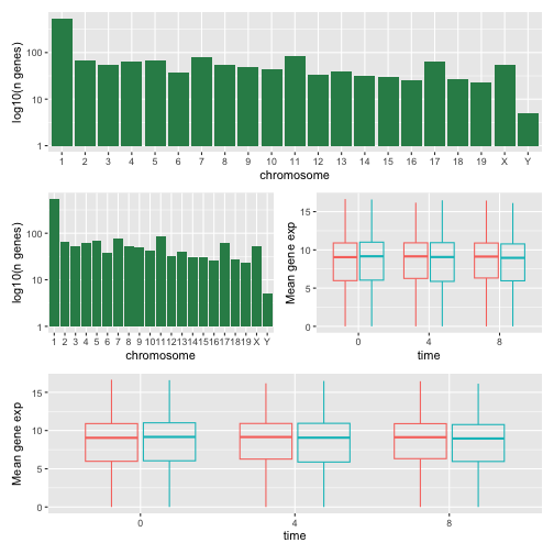
图 49
第 1 张图片,共 1 张:‘A composed figure with the histogram (left) and boxplot (right) side-by-side.’
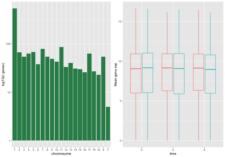
图 50
第 1 张图片,共 1 张:‘The 'base' figures, side-by-side, showing (from left to right) 20 empty dots along the diagonal, same with a vertical red line, and same as the second one with a rectangle overlaid in the middle of the plot.’
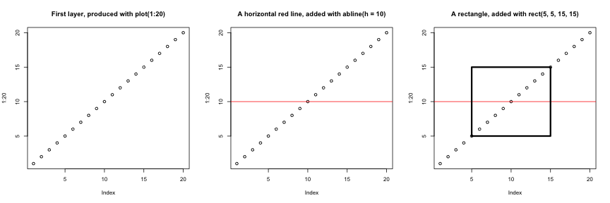
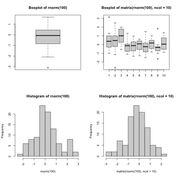
图 51
第 1 张图片,共 1 张:‘A two-by-two composition of 2 boxplots at the top, and 2 histograms at the bottom.’
后续步骤
图 1
第 1 张图片,共 1 张:‘Schematic representation of the SummarizedExperiment class illustrating the following slots: fowData and rowRanges, one assay or multiple assays, colData and metadata.’

图 2
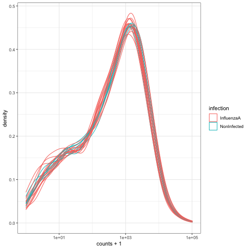
第 1 张图片,共 1 张:‘Density plot showing log of expression counts + 1 density lines, one per samples, coloured based on the infection status.’