Content from RNA-seq入門
Last updated on 2025-11-11 | Edit this page
Estimated time 100 minutes
Overview
Questions
- RNA-seq実験を計画する際に考慮すべきさまざまな選択とは?
- どのように生のfastqファイルを処理して、遺伝子ごと、サンプルごとのリードカウントの表を作成するのですか?
- ある生物についてアノテーションされた遺伝子の情報はどこで見つけることができますか?
- RNA-seq解析の典型的なステップとは?
Objectives
- RNA-seqとは何か?
- RNA-seq実験を実施する前に行わなければならない最も一般的なデザイン選択のいくつかを説明する。
- 生データから下流の解析に使用されるリードカウントマトリックスまでの手順の概要を説明する。
- RNA-seq解析で生成されるいくつかの一般的なタイプの結果と可視化を示す。
RNA-seq実験では何を測定するのか?
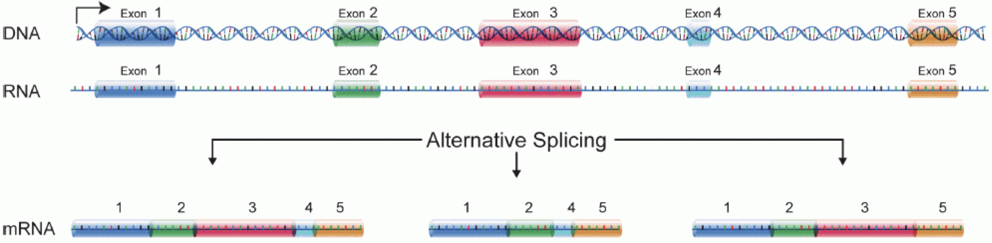
RNA分子を作るには、まずDNAがmRNAに転写される。 その後、イントロン領域がスプライシングされ、エキソン領域が組み合わされて遺伝子の異なる_isoforms_となる。
(図はMartin & Wang (2011)より引用)。
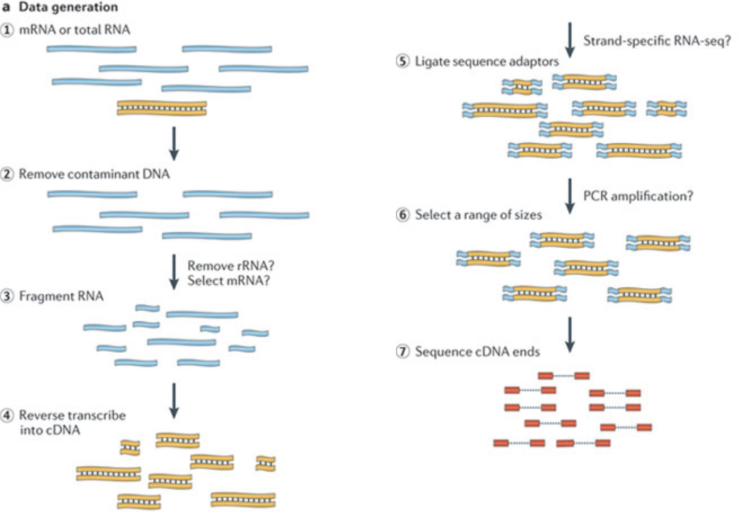
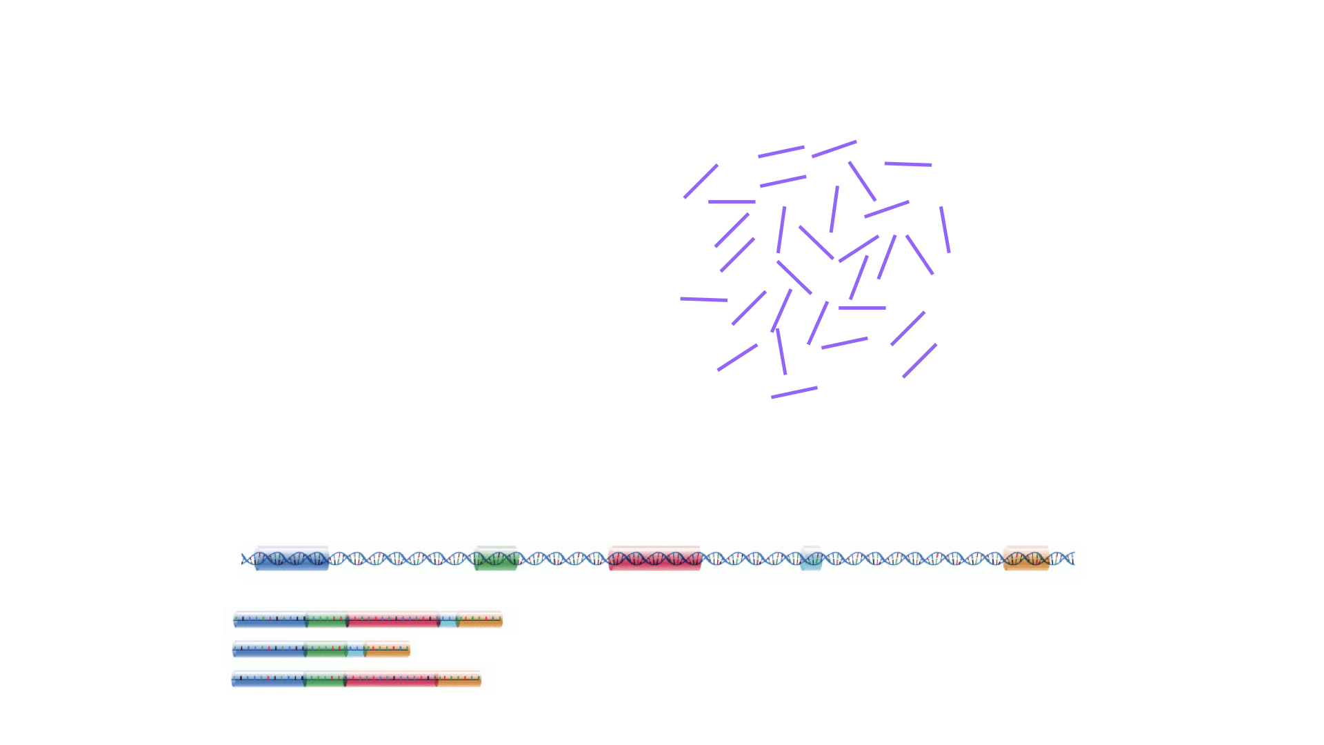
典型的なRNA-seq実験では、まず目的のサンプルからRNA分子を収集する。 ポリA末端を持つ分子(主にmRNA)を濃縮する、あるいは、そうでなければ非常に豊富なリボソームRNAを除去した後、残りの分子を細かく断片化する(分子全体を考慮するロングリード・プロトコルもあるが、このレッスンの焦点ではない)。 イントロン配列を除いたスプライシングのために、RNA分子(したがって生成された断片)はゲノムの途切れることのない領域に対応しない可能性があることを心に留めておくことが重要である。 その後、RNA断片はcDNAに逆転写され、両端に配列決定用アダプターが付加される。 これらのアダプターにより、フラグメントをフローセルに取り付けることができる。 一旦くっつくと、各フラグメントは大きく増幅され、フローセル上に同一配列のクラスターを生成する。 次にシークエンサーは、このようなクラスターに含まれるcDNA断片の最初の50-200塩基の塩基配列を、一端から順に決定する。 多くのデータセットは、両端から断片を読み取る、いわゆるペアエンドプロトコルで作成される。 このようなリード(またはリードのペア)は1回の実験で数百万本生成され、これらは(ペアの)FASTQファイルに表現される。 それぞれのリードは、このようなファイルでは4つの連続した行で表現される。最初に一意のリード識別子の行、次にリードの推定配列、次に別の識別子の行、最後に各推定ヌクレオチドの塩基品質を含む行で、対応する位置のヌクレオチドが正しく同定された確率を表す。
チャレンジ隣人と以下の点について話し合ってください。
- ペアエンドプロトコルの利点と欠点を教えてください。
- リード配列を含むFASTQファイルに対して実行するのに有用な品質評価として、どのようなものが考えられますか?
実験デザインの考察
データ収集を始める前に、実験計画について考える時間を取ることが不可欠である。 実験計画とは、関心のある問題にできるだけ効率的に答えるために、適切な種類のデータと十分な量のデータを確実に入手できるようにすることを目的とした実験の組織に関するものである。 どのような条件や標本群を考慮するか、どれだけの複製を収集するか、実際のデータ収集をどのように計画するかといった側面は、考慮すべき重要な問題である。 多くのハイスループット生物学的実験(RNA-seqを含む)は環境条件に敏感であり、異なる日に、異なる分析者によって、異なるセンターで、異なるバッチの試薬を用いて行われた測定を直接比較することはしばしば困難である。 このため、実験を適切にデザインし、異なるタイプの(一次的効果と二次的効果を)区別できるようにすることが非常に重要である。
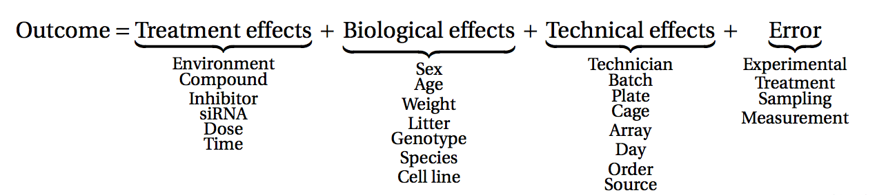
(図はLazic (2017)より)。
チャレンジ隣人と話し合う
- なぜ複製が必要なのですか?
重要なのは、統計学的な観点から見ると、すべての反復が同じように有用というわけではないということである。 後者は通常、測定装置の再現性をテストするために使用され、一方、生物学的な複製は、対象集団からの異なるサンプル間のばらつきについて情報を提供する。 別の方式では、複製(または単位)を「生物学的」、「実験的」、「観察的」に分類する。 ここでいう生物学的単位とは、推論を行いたい実体のことである(動物や人など)。 ある治療法の効果について一般的な見解を述べるには、生物学的単位の再現が必要である。1匹のマウスだけを研究して、マウスの集団に対する薬物の効果について結論を出すことはできない。 実験単位とは、ある処置に独立に割り当てることができる最小の実体である(動物、子、ケージ、井戸など)。 実験単位の再現のみが真の再現となる。 最後に、観測単位とは、測定が行われる実体のことである。
興味のある質問に答える能力に対する実験デザインの影響を調べるために、ConfoundingExplorerパッケージで提供されている対話型アプリケーションを使用する。
チャレンジ
ConfoundingExplorerアプリケーションを起動し、インターフェイスに慣れる。
チャレンジ
- 平衡計画(各バッチの2群間の反復分布が等しい)の場合、バッチ効果の強さを増すとどのような効果がありますか? バッチ効果を調整するかどうかは重要か?
- アンバランスなデザイン(1つのグループのほとんど、またはすべての複製が1つのバッチから得られている)が増えている場合、バッチ効果の強さを増すとどのような影響がありますか? バッチ効果を調整するかどうかは重要か?
RNA-seq定量化:リードからカウントマトリックスまで
シーケンサーからのFASTQファイルに含まれるリード配列は、どの遺伝子や転写産物に由来するかという情報を持っていないため、そのままでは一般的に直接役に立たない。 したがって、最初の処理ステップは、各リードの起源の位置を特定し、これを使用して遺伝子(または個々の転写産物などの別の特徴)に由来するリードの数の推定値を取得しようとするものである。 そして、これを遺伝子の存在量、すなわち発現レベルの代用として用いることができる。 RNA定量パイプラインは数多く存在し、最も一般的なアプローチは主に3つのタイプに分類できる:
リードをゲノムにアライメントし、各遺伝子のエクソン内にマップされたリードの数をカウントする。 これは最もシンプルな方法のひとつだ。 トランスクリプトームのアノテーションが不十分な種については、この方法が望ましい。 例:GRCm39 への
STARアライメント +RsubreadfeatureCountsトランスクリプトームへのリードのアラインメント、トランスクリプトーム発現の定量化、トランスクリプトーム発現を遺伝子発現に要約する。 このアプローチは、正確な定量結果(independent benchmarking)を得ることができる。 、特にDNA汚染のない高品質のサンプルについて。 例GENCODE GRCh38 のトランスクリプトームに対する
rsem-calculate-expression --starとtximportを用いた RSEM 定量化。対応するゲノムをおとりとして、トランスクリプトームに対してリードを疑似整列させ、その過程で転写産物の発現を定量化し、 、転写産物レベルの発現を遺伝子レベルの発現に要約する。 この方法の利点は、計算の効率化、DNA汚染の影響の緩和、GCバイアスの補正などである。 例:
salmon quant --gcBias+tximport
一般的なシーケンスリード深度では、遺伝子発現定量は転写産物発現定量よりも正確であることが多い。 しかし、遺伝子発現の差分解析は、転写産物レベルの定量化にもアクセスすることで、改善 。
RNA-seqの定量に使われる他のツールには以下のようなものがある:TopHat2、bowtie2、kallisto、HTseqなどである。
適切なRNA-seq定量化の選択は、多くの要因の中でも、トランスクリプトームアノテーションの質、 、RNA-seqライブラリー調製の質、コンタミネーション配列の有無に依存する。 多くの場合、複数のアプローチによる定量結果を比較することは有益である。
最適な定量化方法は生物種や実験に依存し、しばしば大量の計算資源を必要とするため、このワークショップではカウントの生成方法に関する具体的な説明は行わない。 その代わりに、上記の参考文献をチェックし、助けが必要であれば地元のバイオインフォマティクスの専門家に相談することをお勧めする。
チャレンジ隣人と以下の点について話し合ってください。
- RNA-Seq定量化ツールについて聞いたことがあるものはどれですか? その他の方法の長所と短所をご存知ですか?
- 独自のRNA-Seq実験を行ったことがありますか? もしそうなら、どのような定量化ツールを使い、なぜそれを選んだのか?
- 定量化のための特定のツール/地元のバイオインフォマティクスの専門家/計算リソースにアクセスできるか? そうでなければ、どうやってアクセスするのか?
参照配列の検索
RNA-seqデータから既知の遺伝子や転写産物の量を定量するためには、これらの特徴の配列を知らせてくれる参照データベースが必要であり、これと我々のリードを比較することができる。 この情報は、さまざまなオンラインレポジトリから得ることができる。 特定のプロジェクトには、異なるソースからの情報を混在させず、これらのうちの1つを選択することを強く推奨する。 選択した定量化ツールによって、必要な参照情報の種類は異なる。 リードをゲノムにアライメントし、既知の注釈付きフィーチャーとのオーバーラップを調べる場合、全ゲノム配列(fastaファイルで提供)と、各注釈付きフィーチャーのゲノム上の位置を示すファイル(通常gtfファイルで提供)が必要です。 リードをトランスクリプトームにマッピングする場合は、代わりに各トランスクリプトの配列を含むファイル(これもfastaファイル)が必要になります。
- マウスやヒトのサンプルを扱う場合、GENCODEプロジェクトは、十分にキュレートされた参照ファイルを提供している。
- Ensemblは、植物や菌類を含む、多数の生物の参照ファイルを提供している。
- また、UCSCは、多くの生物の参照ファイルを提供している。
チャレンジ
GENCODEから最新のマウストランスクリプトームファスタファイルをダウンロードする。
エントリーはどのようなものですか?
ヒント:ファイルをRに読み込むには、Biostrings パッケージの
readDNAStringSet() 関数を使う。
このワークショップで我々はどこに向かっているのか?
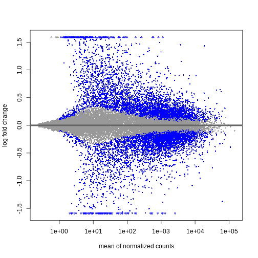
この2日間で、Bioconductorを使ってどのように微分発現解析を行うか、そして結果をどのように解釈するかについて議論し、実践する。 カウントマトリックスから始めるので、最初の品質評価と遺伝子発現の定量はすでに行われていると仮定する。 差次的発現解析の結果は、MAプロットやヒートマップなどのグラフを用いて表現されることが多い(例は下記参照)。

以下のエピソードでは、特にこれらのプロットの作成と解釈の仕方を学ぶ。 また、上位にランクされた遺伝子間に機能的関係があるかどうかを調べるために、遺伝子セット(濃縮)解析と呼ばれるフォローアップ解析を行うことも一般的であるが、これについても後のエピソードで取り上げる。
- RNA-seqは、ある細胞/組織内で発現しているRNAの量と、ある時点での状態を測定する技術である。
- RNA-seq実験を計画する際には、ポリA選択とリボソーム除去のどちらを行うか、ストランドプロトコルとアンストランドプロトコルのどちらを適用するか、シングルエンドとペアエンドのどちらでリードをシーケンスするかなど、多くの選択をしなければならない。 それぞれの選択は、データの処理と解釈に結果をもたらす。
- RNA-seqデータの定量化には多くのアプローチが存在する。 リードをゲノムにアライメントし、遺伝子座にオーバーラップするリードの数をカウントする方法もある。 他の方法は、リードをトランスクリプトームにマッピングし、確率的アプローチを使って各遺伝子や転写産物の存在量を推定する。
- 注釈付き遺伝子に関する情報は、Ensembl、UCSC、GENCODEなどいくつかの情報源からアクセスできる。
Content from RStudioプロジェクトと実験データ
Last updated on 2025-11-11 | Edit this page
Estimated time 30 minutes
Overview
Questions
- RStudioプロジェクトを使用して分析プロジェクトを管理するにはどうすればよいですか?
- 分析プロジェクトのためのディレクトリを効果的に整理する方法は?
- インターネットからデータセットをダウンロードして、ファイルとして保存する方法。
Objectives
- RStudioプロジェクトを作成し、分析プロジェクトに関連するファイルを保存するためのディレクトリを作成します。
- 次のエピソードで使用するデータセットをダウンロードします。
イントロダクション
通常、分析プロジェクトは、データセットファイル、いくつかのRスクリプト、そして出力ファイルが含まれたディレクトリから始まります。
プロジェクトが進むにつれ、より多くのスクリプト、出力ファイルおよびおそらく新しいデータセットの追加により、複雑さは避けられません。
複数のバージョンのスクリプトや出力ファイルを扱う際には、複雑さがさらに増すため、効率的な組織が必要です。
これらが最初からうまく管理されていないと、プロジェクトを休止した後に再開することや、プロジェクトを他の人と共有することは困難かつ時間を要します。
さらに、適切な整理がなければ、プロジェクトの複雑さが頻繁にsetwd関数を使用して異なる作業ディレクトリ間を切り替えることにつながり、無秩序な作業スペースが生じます。
このレッスンでは、最初にデータ分析プロジェクトで使用し生成されたファイルを、_作業ディレクトリ_内で管理するための効果的な戦略に焦点を当てます。
作業ディレクトリとは何ですか?
Rにおける作業ディレクトリは、Rがファイルを読み込んだり保存したりするために探すコンピュータ上のデフォルトの場所です。 詳細は、私たちの データ分析のためのRとBioconductorの紹介 レッスンにあります。
次に、RStudioに組み込まれた分析プロジェクトを管理するための機能であるRStudioプロジェクトを活用する方法を学びます。
RStudioとは何ですか?
RStudioは、科学者やソフトウェア開発者によって広く使われる無料の統合開発環境(IDE)で、ソフトウェアの開発やデータセットの分析に使用されます。 RStudioまたはその一般的な使用に関する支援が必要な場合は、私たちの データ分析のためのRとBioconductorの紹介 レッスンをご参照ください。
最後に、このレッスンでは、次のエピソードのためのデータをダウンロードするためにR関数download.fileを使用する方法も学びます。
作業ディレクトリの構造
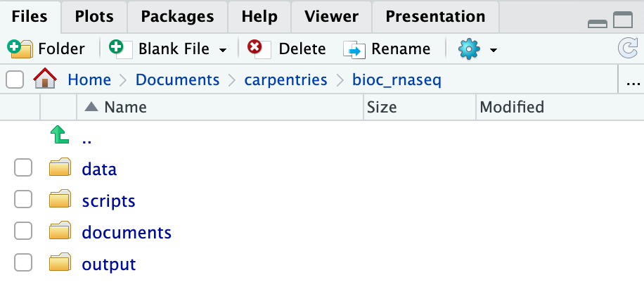
より効率的なワークフローのために、分析に関連付けられたすべてのファイルを特定のディレクトリに保存することをお勧めします。これは、プロジェクトの作業ディレクトリとして機能します。 最初に、この作業ディレクトリには4つの異なるディレクトリが含まれている必要があります:
-
data: 生のデータを格納するために専用。 このフォルダには、生データだけを保存し、データセットが新たに受信されるまで修正しないのが理想的です(それでも、ストレージ容量があれば、将来また必要になる可能性があるため、以前のデータセットも保持することをお勧めします)。 RNA-seqデータ分析の場合、このディレクトリには通常、*.fastqファイルや実験に関連するメタデータファイルが含まれます。 -
scripts: データ分析のために作成したRスクリプトを保存するため。 -
documents: 分析に関連する文書を保存するため。 原稿のアウトラインやチームとのミーティングノートなど。 -
output:scriptsディレクトリ内のRスクリプトによって生成された中間または最終結果を保存するため。 重要なことは、データクリーニングまたは前処理を行う場合、出力はこのディレクトリに保存されるべきであり、これによりもはや生データとは見なされません。
プロジェクトが複雑になるにつれ、追加のディレクトリまたはサブディレクトリを作成する必要があるかもしれません。 それでも、上記の4つのディレクトリは作業ディレクトリの基盤として機能するべきです。
次のエピソードのためのディレクトリを作成する
このエピソードとレッスンの残りの部分のために作業ディレクトリとするために、コンピュータ上にディレクトリを作成します(ワークショップの例ではbio_rnaseqという名前のディレクトリを使用します)。
次に、この選択したディレクトリ内に、前述の4つの基本的なディレクトリ(data、scripts、documents、およびoutput)を作成します。
RStudioプロジェクトを使用して作業ディレクトリを管理する
前述の通り、RStudioプロジェクトは、分析プロジェクトを管理するためにRStudioに組み込まれた機能です。
それは、プロジェクト特有の設定を作業ディレクトリ内に保存された.Rprojファイルに保存することで実現します。
.Rprojファイルを直接開くか、RStudioのプロジェクトを開くオプションを通じてこれらの設定をRStudioにロードすると、Rの作業ディレクトリが.Rprojファイルの場所、すなわちプロジェクトの作業ディレクトリに自動的に設定されます。
RStudioプロジェクトを作成するには:
- RStudioを開始します。
- メニューバーに移動し、
File>New Project...を選択します。 -
Existing Directoryを選択します。 -
Browse...ボタンをクリックし、分析のために以前選択した作業ディレクトリを選択します(つまり、4つの必須ディレクトリが存在するディレクトリ)。 - ウィンドウの右下にある
Create Projectをクリックします。
上記のステップを完了すると、プロジェクトの作業ディレクトリ内に.Rprojファイルが見つかります。
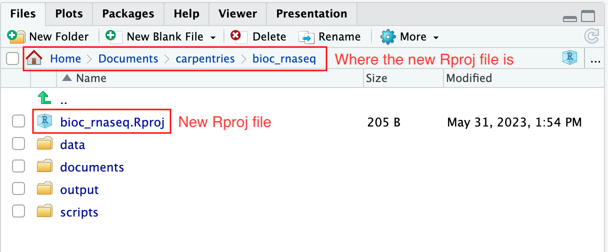
さらに、RStudioコンソールのヘッディングには、.Rprojファイルの存在するプロジェクトの作業ディレクトリの絶対パスが表示されます。RStudioがこのディレクトリをRの作業ディレクトリとして設定したことを示しています。
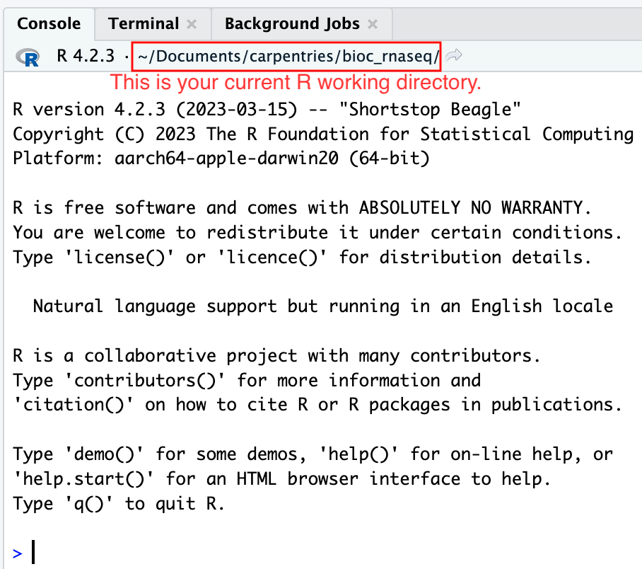
この時点から、読み込むデータがファイルから、またはファイルにデータを保存するRコードを実行すると、それはデフォルトでプロジェクトの作業ディレクトリに相対するパスに向けられます。
プロジェクトを閉じる場合、別のプロジェクトを開くため、新しいプロジェクトを作成するため、またはプロジェクトを一時的に休むためには、メニューバーにあるFile
> Close Projectオプションを使用します。
プロジェクトを再度開くには、作業ディレクトリ内の.Rprojファイルをダブルクリックするか、RStudioを開いてメニューバーのFile
> Open Projectオプションを使用します。
次のエピソードのためにRNA-seqデータをダウンロードする
最後に、私たちは次のエピソードのために必要なRNA-seqデータをダウンロードするためのRの使用方法を学びます。 使用するデータセットは、上気道感染がマウスの小脳および脊髄におけるRNA転写の変化に与える影響を調査するために生成されました。 このデータセットは、次の研究の一部として作成されました:
Blackmore、Stephenら。“インフルエンザ感染は、実験的自己免疫脳脊髄炎の遺伝子モデルにおいて疾患を引き起こします。” 国立科学アカデミー紀要114.30 (2017): E6107-E6116。
データセットはGene Expression Omnibus (GEO)で利用可能で、アクセッション番号はGSE96870です。 GEOからデータをダウンロードすることは簡単ではなく(このレッスンでは扱われません)。 そのため、アクセスが簡単なようにデータをGitHubリポジトリに公表しました。
ファイルをダウンロードするために、私たちはR関数download.fileを使用します。この関数は少なくとも2つのパラメータを必要とします:urlとdestfile。
urlパラメータは、データをダウンロードするためのインターネット上のアドレスを指定するために使用されます。
destfileパラメータは、ダウンロードしたファイルをどこに保存するか、そしてダウンロードしたファイルにどのように名前を付けるかを示します。
このレッスンの残りの部分で必要な4つのデータファイルのうちの1つをダウンロードしてみましょう。
データファイルはhttps://github.com/carpentries-incubator/bioc-rnaseq/raw/main/episodes/data/GSE96870_counts_cerebellum.csvにあります。
ダウンロードしたファイルを作業ディレクトリのdataフォルダにGSE96870_counts_cerebellum.csvという名前で保存します。
R
download.file(
    url = "https://github.com/carpentries-incubator/bioc-rnaseq/raw/main/episodes/data/GSE96870_counts_cerebellum.csv",
    destfile = "data/GSE96870_counts_cerebellum.csv"
)
作業ディレクトリのdataフォルダに移動すると、GSE96870_counts_cerebellum.csvという名前のファイルが見つかるはずです。
残りのデータセットファイルをダウンロードする
このレッスンの残りの部分に必要なデータセットファイルがあと3つあります。
| URL | ファイル名 |
|---|---|
| https://github.com/carpentries-incubator/bioc-rnaseq/raw/main/episodes/data/GSE96870_coldata_cerebellum.csv | GSE96870_coldata_cerebellum.csv |
| https://github.com/carpentries-incubator/bioc-rnaseq/raw/main/episodes/data/GSE96870_coldata_all.csv | GSE96870_coldata_all.csv |
| https://github.com/carpentries-incubator/bioc-rnaseq/raw/main/episodes/data/GSE96870_rowranges.tsv | GSE96870_rowranges.tsv |
download.file関数を使用して、作業ディレクトリのdataフォルダにファイルをダウンロードします。
R
download.file(
    url = "https://github.com/carpentries-incubator/bioc-rnaseq/raw/main/episodes/data/GSE96870_coldata_cerebellum.csv",
    destfile = "data/GSE96870_coldata_cerebellum.csv"
)

download.file(
    url = "https://github.com/carpentries-incubator/bioc-rnaseq/raw/main/episodes/data/GSE96870_coldata_all.csv",
    destfile = "data/GSE96870_coldata_all.csv"
)

download.file(
    url = "https://github.com/carpentries-incubator/bioc-rnaseq/raw/main/episodes/data/GSE96870_rowranges.tsv",
    destfile = "data/GSE96870_rowranges.tsv"
)
- プロジェクトに必要なファイルを作業ディレクトリに適切に整理することは、秩序を維持し、将来のアクセスを容易にするために重要です。
- RStudioプロジェクトは、プロジェクトの作業ディレクトリを管理し、分析を促進するための貴重なツールとして機能します。
- Rにおける
download.file関数は、インターネットからデータセットをダウンロードするために使用できます。
Content from Rに量的データをインポートして注釈を付ける
Last updated on 2025-11-11 | Edit this page
Estimated time 120 minutes
::::::::::::::::::::::::::::::::::::::: objectives
- 量的データをSummarizedExperimentオブジェクトにインポートする方法を学びます。
- オブジェクトに追加の遺伝子注釈を追加する方法を学びます。 ::::::::::::::::::::::::::::::::::::::::::::::::::
:::::::::::::::::::::::::::::::::::::::: questions
- 量的遺伝子発現データをRで下流の統計分析に適したオブジェクトにインポートするにはどうすればよいですか?
- 通常使用される遺伝子識別子の種類は何ですか? それらのマッピングはどのように行われますか? ::::::::::::::::::::::::::::::::::::::::::::::::::
パッケージを読み込む
このエピソードでは、アドオンRパッケージの関数をいくつか使用します。
それらを使用するためには、libraryから読み込む必要があります。
R
suppressPackageStartupMessages({
    library(AnnotationDbi)
    library(org.Mm.eg.db)
    library(hgu95av2.db)
    library(SummarizedExperiment)
})
there is no package called 'XXXX'というエラーメッセージが表示された場合、これはこのバージョンのRに対して、パッケージがまだインストールされていないことを意味します。このワークショップに必要なすべてのパッケージをインストールするには、Summary
and Setupの下部を参照してください。
インストールする必要がある場合は、上記のlibraryコマンドを再実行してそれらを読み込むことを忘れないでください。
データを読み込む
前回のエピソードでは、Rを使用してインターネットから4つのファイルをダウンロードし、それらをコンピュータに保存しました。 しかし、これらのファイルはまだRに読み込まれていないため、作業することができません。 Blackmore et al. 2017の元の実験デザインはかなり複雑でした。8週齢のオスとメスのC57BL/6マウスは、インフルエンザ感染前の0日目、感染後の4日目および8日目に収集されました。 各マウスからは、小脳と脊髄の組織がRNA-seq用に取り出されました。 元々は「性別 x 時間 x 組織」群御に4匹のマウスがいましたが、途中でいくつかが失われ、合計で45のサンプルに至りました。 このワークショップでは、分析を簡素化するために22の小脳サンプルのみを使用します。 発現の定量化は、STARを使用してマウスのゲノムにアライメントを行い、その後、遺伝子にマッピングされるリードの数を数えることを通じて行われました。 各遺伝子ごとのサンプルあたりのカウントに加えて、どのサンプルがどの性別/時間点/複製に属するかの情報も必要です。 遺伝子に関しては、注釈と呼ばれる追加の情報があると便利です。 前回ダウンロードしたデータファイルを読み込み、探索し始めましょう:
カウント
R
counts <- read.csv("data/GSE96870_counts_cerebellum.csv",
                   row.names = 1)
dim(counts)
OUTPUT
[1] 41786 22R
# View(counts)
遺伝子は行に、サンプルは列に含まれています。したがって、41,786の遺伝子と22のサンプルのカウントがあります。
View()コマンドはウェブサイト用にコメントアウトされていますが、実行するとRStudioでデータを確認したり、特定の列でテーブルを並べ替えたりできます。
ただし、ビューワはcountsオブジェクト内部のデータを変更できないため、見るだけで、永久に並べ替えたり編集したりすることはできません。
終了したら、タブのXを使ってビューワを閉じます。
行名は遺伝子シンボルであり、列名はGEOのサンプルIDであるようです。これは、私たちがどのサンプルが何かを教えてくれないため、あまり有益ではありません。
サンプルの注釈
次に、サンプルの注釈を読み込みます。
カウント行列の列にはサンプルが含まれているため、オブジェクトにcoldataという名前を付けます:
R
coldata <- read.csv("data/GSE96870_coldata_cerebellum.csv",
                    row.names = 1)
dim(coldata)
OUTPUT
[1] 22 10R
# View(coldata)
今、サンプルが行にあり、GEOサンプルIDが行名として付いています。そして、私たちには10列の情報があります。
このワークショップで最も便利な列は、geo_accession(再度、GEOサンプルID)、sex、およびtimeです。
遺伝子の注釈
カウントには遺伝子シンボルしかありませんが、それは短くて人間の脳にとってはある程度認識可能ですが、実際に測定された遺伝子の正確な同定子としてはあまり利便性がありません。
そのため、著者によって提供された追加の遺伝子注釈が必要です。
countおよびcoldataファイルはカンマ区切り値(.csv)形式でしたが、遺伝子注釈ファイルにはそれが使用できません。なぜなら、説明には、カンマを含む可能性があるため、.csvファイルを正しく読み込むのを妨げるからです。
その代わりに、遺伝子注釈ファイルはタブ区切り値(.tsv)形式です。
同様に、説明には単一引用符'(例:5’)が含まれる可能性があり、Rはデフォルトでこれを文字列として扱うためです。
そのため、データがタブ区切りであることを指定するために、より一般的な関数read.delim()に追加の引数を使用する必要があります(sep = "\t")で、引用符は使用しない(quote = "")。
さらに、最初の行に列名が含まれていることを指定するためにその他の引数を追加し(header = TRUE)、行名として指定される遺伝子シンボルは5列目(row.names = 5)であること、NCBIの種特異的遺伝子ID(すなわちENTREZID)は、数字のように見えるが文字列として読み込む(colClasses引数)必要があることを指定します。
使用可能な引数に関する詳細については、関数名の先頭にクエスチョンマークを入力することで確認できます。
(例:?read.delim)
R
rowranges <- read.delim("data/GSE96870_rowranges.tsv",
                        sep = "\t",
                        colClasses = c(ENTREZID = "character"),
                        header = TRUE,
                        quote = "",
                        row.names = 5)
dim(rowranges)
OUTPUT
[1] 41786 7R
# View(rowranges)
41,786の遺伝子ごとに、seqnames(例えば、染色体数)、startおよびend位置、strand、ENTREZID、遺伝子産物説明(product)および特徴タイプ(gbkey)があります。
これらの遺伝子レベルのメタデータは、下流分析に役立ちます。
たとえば、gbkey列から、どのような種類の遺伝子があり、それらがデータセットにどのくらい含まれているかを確認できます:
R
table(rowranges$gbkey)
OUTPUT
     C_region     D_segment          exon     J_segment      misc_RNA
           20            23          4008            94          1988
         mRNA         ncRNA precursor_RNA          rRNA          tRNA
        21198         12285          1187            35           413
    V_segment
535 チャレンジ: 以下のポイントを隣の人と話し合ってください。
-
counts、coldata、rowrangesの3つのオブジェクトは、行および列に関してどのように関連していますか? - mRNA遺伝子のみを分析したい場合、一般的にはどのようにしてそれらだけを保持しますか?(正確なコードではない)
- 最初の2つのサンプルが外れ値であると印象付ける場合、それらを削除するにはどうすればよいですか?(一般的には、正確なコードではない)
-
countsでは、行は遺伝子であり、rowrangesの行と同じです。countsの列はサンプルですが、これはcoldataの行に対応します。 -
countsの行をmRNA遺伝子に限定し、rowrangesの行もそのようにしなければなりません。 -
countsの列とcoldataの行で、最初の2つのサンプルを除外するために両方の行をサブセットする必要があります。
関連情報を別のオブジェクトに保持することで、カウント、遺伝子の注釈、サンプルの注釈の間で不一致が発生する可能性があります。
これが、BioconductorがSummarizedExperimentという特殊なS4クラスを作成した理由です。
SummarizedExperimentの詳細は、RNA解析とBioconductorの導入ワークショップの最後で詳しく説明されています。
リマインダーとして、SummarizedExperimentクラスの構造を表す図を見てみましょう:

これは、任意の種類の定量的なオミクスデータ(assays)と、それにリンクされたサンプル注釈(colData)、および(遺伝子)特徴注釈(rowRanges)または染色体、開始および終了位置を持たない(rowData)形式で保持されるように設計されています。
これらの3つのテーブルが(正しく)リンクされると、サンプルや特徴の部分集合がassay、colData、rowRangesの正しい部分集合に変わります。
さらに、ほとんどのBioconductorパッケージは同じコアデータインフラストラクチャに基づいて構築されているため、SummarizedExperimentオブジェクトを認識し、操作することができます。
さらに、ほとんどのBioconductorパッケージは同じコアデータインフラストラクチャの周りに構築されているため、SummarizedExperimentオブジェクトを認識し、操作できるようになります。
最も人気のある2つのRNA-seq統計分析パッケージは、統計結果用に追加のスロットがあるSummarizedExperimentに類似した独自の拡張S4クラスを持っています:DESeq2のDESeqDataSetおよびedgeRのDGEListです。
統計分析に使用するものが何であれ、データをSummarizedExperimentに入れることから始めることができます。
SummarizedExperimentを組み立てる
これらのオブジェクトからSummarizedExperimentを作成します。
-
countオブジェクトはassaysスロットに保存されます。 - サンプル情報を持つ
coldataオブジェクトは、colDataスロットに保存されます(サンプルメタデータ) - 遺伝子を記述する
rowrangesオブジェクトは、rowRangesスロットに保存されます(特徴メタデータ)
それらを組み合わせる前に、サンプルと遺伝子が同じ順序であることを絶対に確認する必要があります!
countとcoldataが同じ数のサンプルを持っていること、またcountとrowrangesが同じ数の遺伝子を持っていることはわかりましたが、同じ順序になっているかどうかを明示的に確認することはしていませんでした。
確認する簡単な方法:
R
all.equal(colnames(counts), rownames(coldata)) # samples
OUTPUT
[1] TRUER
all.equal(rownames(counts), rownames(rowranges)) # genes
OUTPUT
[1] TRUER
# 最初がTRUEでない場合は、このようにしてカウントのサンプル/列をコレクトします(これは最初がTRUEでも実行しても構いません):

tempindex <- match(colnames(counts), rownames(coldata))
coldata <- coldata[tempindex, ]

# 再確認します:
all.equal(colnames(counts), rownames(coldata))
OUTPUT
[1] TRUEChallenge
アッセイ(例:counts)および遺伝子注釈テーブル(例:rowranges)内の特徴(すなわち遺伝子)が異なる場合、これらをどのように修正できますか?
コードを記述してください。
R
tempindex <- match(rownames(counts), rownames(rowranges))
rowranges <- rowranges[tempindex, ]

all.equal(rownames(counts), rownames(rowranges))
サンプルと遺伝子が同じ順序になっていることを確認したら、SummarizedExperimentオブジェクトを作成します。
R
# 最後の確認:
stopifnot(rownames(rowranges) == rownames(counts), # features
          rownames(coldata) == colnames(counts)) # samples

se <- SummarizedExperiment(
    assays = list(counts = as.matrix(counts)),
    rowRanges = as(rowranges, "GRanges"),
    colData = coldata
)
遺伝子とサンプルが一致していることが非常に重要であるため、SummarizedExperiment()コンストラクタは内部で一致する遺伝子/サンプル数とサンプル/行名が一致することをチェックします。
そうでない場合、いくつかのエラーメッセージが表示されます:
R
# サンプル数の誤り:

bad1 <- SummarizedExperiment(
    assays = list(counts = as.matrix(counts)),
    rowRanges = as(rowranges, "GRanges"),
    colData = coldata[1:3,]
)
ERROR
Error in validObject(.Object): invalid class "SummarizedExperiment" object:
    nb of cols in 'assay' (22) must equal nb of rows in 'colData' (3)
R
# 同じ数の遺伝子ですが異なる順序:

bad2 <- SummarizedExperiment(
  assays = list(counts = as.matrix(counts)),
  rowRanges = as(rowranges[c(2:nrow(rowranges), 1),], "GRanges"),
  colData = coldata
)
ERROR
Error in SummarizedExperiment(assays = list(counts = as.matrix(counts)), : the rownames and colnames of the supplied assay(s) must be NULL or identical
  to those of the RangedSummarizedExperiment object (or derivative) to
constructSummarizedExperimentのさまざまなデータスロットにアクセスする方法と、いくつかの操作を行う方法の簡単な概要:
R
# カウントにアクセス
head(assay(se))
OUTPUT
             GSM2545336 GSM2545337 GSM2545338 GSM2545339 GSM2545340 GSM2545341
Xkr4               1891       2410       2159       1980       1977       1945
LOC105243853          0          0          1          4          0          0
LOC105242387        204        121        110        120        172        173
LOC105242467         12          5          5          5          2          6
Rp1                   2          2          0          3          2          1
Sox17               251        239        218        220        261        232
             GSM2545342 GSM2545343 GSM2545344 GSM2545345 GSM2545346 GSM2545347
Xkr4               1757       2235       1779       1528       1644       1585
LOC105243853          1          3          3          0          1          3
LOC105242387        177        130        131        160        180        176
LOC105242467          3          2          2          2          1          2
Rp1                   3          1          1          2          2          2
Sox17               179        296        233        271        205        230
             GSM2545348 GSM2545349 GSM2545350 GSM2545351 GSM2545352 GSM2545353
Xkr4               2275       1881       2584       1837       1890       1910
LOC105243853          1          0          0          1          1          0
LOC105242387        161        154        124        221        272        214
LOC105242467          2          4          7          1          3          1
Rp1                   3          6          5          3          5          1
Sox17               302        286        325        201        267        322
             GSM2545354 GSM2545362 GSM2545363 GSM2545380
Xkr4               1771       2315       1645       1723
LOC105243853          0          1          0          1
LOC105242387        124        189        223        251
LOC105242467          4          2          1          4
Rp1                   3          3          1          0
Sox17               273        197        310        246
R
dim(assay(se))
OUTPUT
[1] 41786 22R
# 上記は、私たちが今持っているのが1つのアッセイ、"counts"のために機能しています。
# しかし、アッセイが複数ある場合は、指定する必要があります。
# 例えば、

head(assay(se, "counts"))
OUTPUT
             GSM2545336 GSM2545337 GSM2545338 GSM2545339 GSM2545340 GSM2545341
Xkr4               1891       2410       2159       1980       1977       1945
LOC105243853          0          0          1          4          0          0
LOC105242387        204        121        110        120        172        173
LOC105242467         12          5          5          5          2          6
Rp1                   2          2          0          3          2          1
Sox17               251        239        218        220        261        232
             GSM2545342 GSM2545343 GSM2545344 GSM2545345 GSM2545346 GSM2545347
Xkr4               1757       2235       1779       1528       1644       1585
LOC105243853          1          3          3          0          1          3
LOC105242387        177        130        131        160        180        176
LOC105242467          3          2          2          2          1          2
Rp1                   3          1          1          2          2          2
Sox17               179        296        233        271        205        230
             GSM2545348 GSM2545349 GSM2545350 GSM2545351 GSM2545352 GSM2545353
Xkr4               2275       1881       2584       1837       1890       1910
LOC105243853          1          0          0          1          1          0
LOC105242387        161        154        124        221        272        214
LOC105242467          2          4          7          1          3          1
Rp1                   3          6          5          3          5          1
Sox17               302        286        325        201        267        322
             GSM2545354 GSM2545362 GSM2545363 GSM2545380
Xkr4               1771       2315       1645       1723
LOC105243853          0          1          0          1
LOC105242387        124        189        223        251
LOC105242467          4          2          1          4
Rp1                   3          3          1          0
Sox17               273        197        310        246
R
# サンプル注釈にアクセス
colData(se)
OUTPUT
DataFrame with 22 rows and 10 columns
                     title geo_accession     organism         age         sex
               <character>   <character>  <character> <character> <character>
GSM2545336 CNS_RNA-seq_10C    GSM2545336 Mus musculus     8 weeks      Female
GSM2545337 CNS_RNA-seq_11C    GSM2545337 Mus musculus     8 weeks      Female
GSM2545338 CNS_RNA-seq_12C    GSM2545338 Mus musculus     8 weeks      Female
GSM2545339 CNS_RNA-seq_13C    GSM2545339 Mus musculus     8 weeks      Female
GSM2545340 CNS_RNA-seq_14C    GSM2545340 Mus musculus     8 weeks        Male
...                    ...           ...          ...         ...         ...
GSM2545353  CNS_RNA-seq_3C    GSM2545353 Mus musculus     8 weeks      Female
GSM2545354  CNS_RNA-seq_4C    GSM2545354 Mus musculus     8 weeks        Male
GSM2545362  CNS_RNA-seq_5C    GSM2545362 Mus musculus     8 weeks      Female
GSM2545363  CNS_RNA-seq_6C    GSM2545363 Mus musculus     8 weeks        Male
GSM2545380  CNS_RNA-seq_9C    GSM2545380 Mus musculus     8 weeks      Female
             infection      strain        time      tissue     mouse
           <character> <character> <character> <character> <integer>
GSM2545336  InfluenzaA     C57BL/6        Day8  Cerebellum        14
GSM2545337 NonInfected     C57BL/6        Day0  Cerebellum         9
GSM2545338 NonInfected     C57BL/6        Day0  Cerebellum        10
GSM2545339  InfluenzaA     C57BL/6        Day4  Cerebellum        15
GSM2545340  InfluenzaA     C57BL/6        Day4  Cerebellum        18
...                ...         ...         ...         ...       ...
GSM2545353 NonInfected     C57BL/6        Day0  Cerebellum         4
GSM2545354 NonInfected     C57BL/6        Day0  Cerebellum         2
GSM2545362  InfluenzaA     C57BL/6        Day4  Cerebellum        20
GSM2545363  InfluenzaA     C57BL/6        Day4  Cerebellum        12
GSM2545380  InfluenzaA     C57BL/6        Day8  Cerebellum        19
R
dim(colData(se))
OUTPUT
[1] 22 10R
# 遺伝子注釈にアクセス
head(rowData(se))
OUTPUT
DataFrame with 6 rows and 3 columns
                ENTREZID                product       gbkey
             <character>            <character> <character>
Xkr4              497097 X Kell blood group p..        mRNA
LOC105243853   105243853 uncharacterized LOC1..       ncRNA
LOC105242387   105242387 uncharacterized LOC1..       ncRNA
LOC105242467   105242467 lipoxygenase homolog..        mRNA
Rp1                19888 retinitis pigmentosa..        mRNA
Sox17              20671 SRY (sex determining..        mRNA
R
dim(rowData(se))
OUTPUT
[1] 41786 3R
# 性別、時間、マウスIDを表示するためのより良いサンプルIDを作成します:

se$Label <- paste(se$sex, se$time, se$mouse, sep = "_")
se$Label
OUTPUT
 [1] "Female_Day8_14" "Female_Day0_9"  "Female_Day0_10" "Female_Day4_15"
 [5] "Male_Day4_18"   "Male_Day8_6"    "Female_Day8_5"  "Male_Day0_11"
 [9] "Female_Day4_22" "Male_Day4_13"   "Male_Day8_23"   "Male_Day8_24"
[13] "Female_Day0_8"  "Male_Day0_7"    "Male_Day4_1"    "Female_Day8_16"
[17] "Female_Day4_21" "Female_Day0_4"  "Male_Day0_2"    "Female_Day4_20"
[21] "Male_Day4_12"   "Female_Day8_19"
R
colnames(se) <- se$Label

# サンプルは性別と時間に基づいて並んでいません。
se$Group <- paste(se$sex, se$time, sep = "_")
se$Group
OUTPUT
 [1] "Female_Day8" "Female_Day0" "Female_Day0" "Female_Day4" "Male_Day4"
 [6] "Male_Day8"   "Female_Day8" "Male_Day0"   "Female_Day4" "Male_Day4"
[11] "Male_Day8"   "Male_Day8"   "Female_Day0" "Male_Day0"   "Male_Day4"
[16] "Female_Day8" "Female_Day4" "Female_Day0" "Male_Day0"   "Female_Day4"
[21] "Male_Day4"   "Female_Day8"
R
# これを順序を保持するファクターデータに変更し、seオブジェクトを再配置します:

se$Group <- factor(se$Group, levels = c("Female_Day0","Male_Day0",
                                        "Female_Day4","Male_Day4",
                                        "Female_Day8","Male_Day8"))
se <- se[, order(se$Group)]
colData(se)
OUTPUT
DataFrame with 22 rows and 12 columns
                         title geo_accession     organism         age
                   <character>   <character>  <character> <character>
Female_Day0_9  CNS_RNA-seq_11C    GSM2545337 Mus musculus     8 weeks
Female_Day0_10 CNS_RNA-seq_12C    GSM2545338 Mus musculus     8 weeks
Female_Day0_8  CNS_RNA-seq_27C    GSM2545348 Mus musculus     8 weeks
Female_Day0_4   CNS_RNA-seq_3C    GSM2545353 Mus musculus     8 weeks
Male_Day0_11   CNS_RNA-seq_20C    GSM2545343 Mus musculus     8 weeks
...                        ...           ...          ...         ...
Female_Day8_16  CNS_RNA-seq_2C    GSM2545351 Mus musculus     8 weeks
Female_Day8_19  CNS_RNA-seq_9C    GSM2545380 Mus musculus     8 weeks
Male_Day8_6    CNS_RNA-seq_17C    GSM2545341 Mus musculus     8 weeks
Male_Day8_23   CNS_RNA-seq_25C    GSM2545346 Mus musculus     8 weeks
Male_Day8_24   CNS_RNA-seq_26C    GSM2545347 Mus musculus     8 weeks
                       sex   infection      strain        time      tissue
               <character> <character> <character> <character> <character>
Female_Day0_9       Female NonInfected     C57BL/6        Day0  Cerebellum
Female_Day0_10      Female NonInfected     C57BL/6        Day0  Cerebellum
Female_Day0_8       Female NonInfected     C57BL/6        Day0  Cerebellum
Female_Day0_4       Female NonInfected     C57BL/6        Day0  Cerebellum
Male_Day0_11          Male NonInfected     C57BL/6        Day0  Cerebellum
...                    ...         ...         ...         ...         ...
Female_Day8_16      Female  InfluenzaA     C57BL/6        Day8  Cerebellum
Female_Day8_19      Female  InfluenzaA     C57BL/6        Day8  Cerebellum
Male_Day8_6           Male  InfluenzaA     C57BL/6        Day8  Cerebellum
Male_Day8_23          Male  InfluenzaA     C57BL/6        Day8  Cerebellum
Male_Day8_24          Male  InfluenzaA     C57BL/6        Day8  Cerebellum
                   mouse          Label       Group
               <integer>    <character>    <factor>
Female_Day0_9          9  Female_Day0_9 Female_Day0
Female_Day0_10        10 Female_Day0_10 Female_Day0
Female_Day0_8          8  Female_Day0_8 Female_Day0
Female_Day0_4          4  Female_Day0_4 Female_Day0
Male_Day0_11          11   Male_Day0_11 Male_Day0
...                  ...            ...         ...
Female_Day8_16        16 Female_Day8_16 Female_Day8
Female_Day8_19        19 Female_Day8_19 Female_Day8
Male_Day8_6            6    Male_Day8_6 Male_Day8
Male_Day8_23          23   Male_Day8_23 Male_Day8
Male_Day8_24          24   Male_Day8_24 Male_Day8
R
# 最後に、プロット内での順序を維持するためにLabel列もファクタにします:

se$Label <- factor(se$Label, levels = se$Label)
Challenge
-
Infection変数の各レベルに対して、サンプルは何個ですか? -
se_infectedとse_noninfectedという名前の2つのオブジェクトを作成し、それぞれに感染サンプルと非感染サンプルのみを含むseのサブセットを含めます。 その後、最初の500遺伝子の各オブジェクトの平均発現レベルを計算し、summary()関数を使用してこれらの遺伝子に基づく感染と非感染サンプルの発現レベルの分布を調べます。 - インフルエンザAに感染した雌のマウスのサンプルは何個ありますか?
R
# 1
table(se$infection)
OUTPUT
 InfluenzaA NonInfected
         15           7
R
# 2
se_infected <- se[, se$infection == "InfluenzaA"]
se_noninfected <- se[, se$infection == "NonInfected"]

means_infected <- rowMeans(assay(se_infected)[1:500, ])
means_noninfected <- rowMeans(assay(se_noninfected)[1:500, ])

summary(means_infected)
OUTPUT
     Min.   1st Qu.    Median      Mean   3rd Qu.      Max.
0.000e+00 1.333e-01 2.867e+00 7.641e+02 3.374e+02 1.890e+04
R
summary(means_noninfected)
OUTPUT
     Min.   1st Qu.    Median      Mean   3rd Qu.      Max.
0.000e+00 1.429e-01 3.143e+00 7.710e+02 3.666e+02 2.001e+04
R
# 3
ncol(se[, se$sex == "Female" & se$infection == "InfluenzaA" & se$time == "Day8"])
OUTPUT
[1] 4SummarizedExperimentを保存する
これが、私たちのSummarizedExperimentオブジェクトを作成するための少しのコードと時間でした。
ワークショップ全体で使用し続ける必要があるため、Rのメモリに戻すためにコンピュータ上の実際の単一ファイルとして保存することが有用です。
Rに特有のファイルを保存するには、saveRDS()関数を使用し、後でreadRDS()関数を使用して再び読み込むことができます。
R
saveRDS(se, "data/GSE96870_se.rds")
rm(se) # オブジェクトを削除!
se <- readRDS("data/GSE96870_se.rds")
データの由来と再現性
これで、RNA-SeqデータをRにインポートしてさまざまなパッケージによる分析で使用可能な形式の外部.rdsファイルを作成しました。 ただし、インターネットからダウンロードした3つのファイルから.rdsファイルを作成するために使用したコードの記録を保持する必要があります。 ファイルの由来はどうなっていますか? つまり、それらはどこから来ており、どのように作成されたのですか? 元々のカウントおよび遺伝子情報は、GEO公開データベースに預けられました。アクセッション番号はGSE96870です。 ただし、これらのカウントは、配列ベースコールや品質スコアを保持するファストqファイルで配列合わせ/定量化プログラムを実行することによって生成されたものであり、これらは特定のライブラリ調製法を使用して抽出されたRNAから収集したサンプルで生成されたものです。 ふぅ!
元の実験を実施した場合、理想的にはデータが生成された場所と方法の完全な記録を持つべきです。
しかし、公開データセットを利用している場合、最善の方法は、どの元のファイルがどこから来たか、そしてそれに対して行ってきた操作の記録を保持することです。
Rコードを使用してすべてを追跡することは、元の入力ファイルから全体の分析を再現可能にする素晴らしい方法です。
得られる正確な結果は、Rのバージョン、アドオンパッケージのバージョン、さらには使用しているオペレーティングシステムによって異なる可能性があるため、sessionInfo()を使用してすべての情報を追跡し、出力を記録するようにしてください(レッスンの最後に例を参照)。
チャレンジ: mRNA遺伝子をサブセットにする方法
以前は、mRNA遺伝子に対するサブセットを理論的に論じました。
現在、SummarizedExperimentオブジェクトを持っているため、seを新しいオブジェクトse_mRNAにサブセットするためのコードを書くことがはるかに簡単になります。このオブジェクトには、rowData(se)$gbkeyがmRNAである遺伝子/行のみを含むものです。
コードを書くと、21,198のmRNA遺伝子を正しく取得したかを確認してください。
R
se_mRNA <- se[rowData(se)$gbkey == "mRNA" , ]
dim(se_mRNA)
OUTPUT
[1] 21198 22遺伝子注釈
カウントデータを生成する人によっては、追加の遺伝子注釈の適切なファイルがないかもしれません。 遺伝子シンボルやENTREZID、あるいは他のデータベースのIDのみが存在するかもしれません。 遺伝子注釈の特性は、その注釈戦略と情報源によって異なります。 たとえば、RefSeqヒト遺伝子モデル(つまり、NCBIのEntrez)は、さまざまな研究でよくサポートされ、広く使用されています。 UCSC Known Genes データセットは、Swiss-Prot/TrEMBL (UniProt) のタンパク質データと、GenBankからの関連するmRNAデータに基づいており、UCSC Genome Browserの基盤として機能します。 Ensemblの遺伝子は、自動生成されたゲノムアノテーションと手動キュレーションの両方を含んでいます。
Bioconductorでの詳細情報は、Annotation Workshopの資料で見つけることができます。
Bioconductorには、遺伝子の追加注釈情報を取得するための多くのパッケージや関数があります。 利用可能なリソースについては、エピソード7 遺伝子セット濃縮解析で詳しく説明されています。
ここでは、遺伝子IDマッピング関数の1つであるmapIdsを紹介します:
mapIds(annopkg, keys, column, keytype, ..., multiVals)どこで
- _annopkg_は、注釈パッケージです
- _keys_は、私たちが知っているIDです
- _column_は、私たちが望む値です
- _keytype_は、使用するキーのタイプです
R
mapIds(org.Mm.eg.db, keys = "497097", column = "SYMBOL", keytype = "ENTREZID")
OUTPUT
'select()' returned 1:1 mapping between keys and columnsOUTPUT
497097
"Xkr4" select()関数とは異なり、mapIds()関数は、追加の引数multiValsを通じてキーと列の間の1:多のマッピングを処理します。
以下の例では、hgu95av2.dbパッケージを使用してこの機能を示します。AffymetrixヒトゲノムU95セット注釈データ。
R
keys <- head(keys(hgu95av2.db, "ENTREZID"))
last <- function(x){x[[length(x)]]}

mapIds(hgu95av2.db, keys = keys, column = "ALIAS", keytype = "ENTREZID")
OUTPUT
'select()' returned 1:many mapping between keys and columnsOUTPUT
       10       100      1000     10000 100008586     10001
   "AAC2"    "ADA1"   "ACOGS"    "MPPH"     "AL4"   "ARC33"
R
# 1:多のマッピングがある場合、デフォルトの動作は最初の一致を出力することでした。これは、上で定義した関数を使用して最後の一致を取得するように変更できます:

mapIds(hgu95av2.db, keys = keys, column = "ALIAS", keytype = "ENTREZID", multiVals = last)
OUTPUT
'select()' returned 1:many mapping between keys and columnsOUTPUT
       10       100      1000     10000 100008586     10001
   "NAT2"     "ADA"    "CDH2"    "AKT3" "GAGE12F"    "MED6"
R
# または、すべての多くのマッピングを取得することができます:

mapIds(hgu95av2.db, keys = keys, column = "ALIAS", keytype = "ENTREZID", multiVals = "list")
OUTPUT
'select()' returned 1:many mapping between keys and columnsOUTPUT
$`10`
[1] "AAC2"  "NAT-2" "PNAT"  "NAT2"

$`100`
[1] "ADA1" "ADA"

$`1000`
[1] "ACOGS"  "ADHD8"  "ARVD14" "CD325"  "CDHN"   "CDw325" "NCAD"   "CDH2"

$`10000`
[1] "MPPH"         "MPPH2"        "PKB-GAMMA"    "PKBG"         "PRKBG"
[6] "RAC-PK-gamma" "RAC-gamma"    "STK-2"        "AKT3"

$`100008586`
[1] "AL4"     "CT4.7"   "GAGE-7"  "GAGE-7B" "GAGE-8"  "GAGE7"   "GAGE7B"
[8] "GAGE12F"

$`10001`
[1] "ARC33"     "NY-REN-28" "MED6"
セッション情報
R
sessionInfo()
OUTPUT
R version 4.5.2 (2025-10-31)
Platform: x86_64-pc-linux-gnu
Running under: Ubuntu 22.04.5 LTS

Matrix products: default
BLAS:   /usr/lib/x86_64-linux-gnu/blas/libblas.so.3.10.0
LAPACK: /usr/lib/x86_64-linux-gnu/lapack/liblapack.so.3.10.0  LAPACK version 3.10.0

locale:
 [1] LC_CTYPE=C.UTF-8       LC_NUMERIC=C           LC_TIME=C.UTF-8
 [4] LC_COLLATE=C.UTF-8     LC_MONETARY=C.UTF-8    LC_MESSAGES=C.UTF-8
 [7] LC_PAPER=C.UTF-8       LC_NAME=C              LC_ADDRESS=C
[10] LC_TELEPHONE=C         LC_MEASUREMENT=C.UTF-8 LC_IDENTIFICATION=C

time zone: UTC
tzcode source: system (glibc)

attached base packages:
[1] stats4    stats     graphics  grDevices utils     datasets  methods
[8] base

other attached packages:
 [1] hgu95av2.db_3.13.0          org.Hs.eg.db_3.21.0
 [3] org.Mm.eg.db_3.21.0         AnnotationDbi_1.70.0
 [5] SummarizedExperiment_1.38.1 Biobase_2.68.0
 [7] MatrixGenerics_1.20.0       matrixStats_1.5.0
 [9] GenomicRanges_1.60.0        GenomeInfoDb_1.44.1
[11] IRanges_2.42.0              S4Vectors_0.46.0
[13] BiocGenerics_0.54.0         generics_0.1.4
[15] knitr_1.50

loaded via a namespace (and not attached):
 [1] renv_1.1.5              SparseArray_1.8.1       xml2_1.4.1
 [4] RSQLite_2.4.2           lattice_0.22-7          tinkr_0.3.0
 [7] magrittr_2.0.4          evaluate_1.0.4          grid_4.5.2
[10] fastmap_1.2.0           blob_1.2.4              jsonlite_2.0.0
[13] Matrix_1.7-3            processx_3.8.6          DBI_1.2.3
[16] ps_1.9.1                BiocManager_1.30.26     httr_1.4.7
[19] purrr_1.2.0             UCSC.utils_1.4.0        Biostrings_2.76.0
[22] abind_1.4-8             cli_3.6.5               rlang_1.1.6
[25] crayon_1.5.3            XVector_0.48.0          bit64_4.6.0-1
[28] cachem_1.1.0            withr_3.0.2             DelayedArray_0.34.1
[31] yaml_2.3.10             S4Arrays_1.8.1          tools_4.5.2
[34] sandpaper_0.17.2.9000   memoise_2.0.1           GenomeInfoDbData_1.2.14
[37] assertthat_0.2.1        png_0.1-8               vctrs_0.6.5
[40] R6_2.6.1                lifecycle_1.0.4         KEGGREST_1.48.1
[43] bit_4.6.0               pkgconfig_2.0.3         callr_3.7.6
[46] glue_1.8.0              xfun_0.52               pegboard_0.7.9
[49] compiler_4.5.2
::: keypoints
- 使用される遺伝子発現定量ツールによって、出力を
SummarizedExperimentまたはDGEListオブジェクトに読み込む方法が異なります(多くはBioconductorパッケージで配布されています)。 - EnsemblやEntrez IDなどの安定した遺伝子識別子は、RNA-seq分析全体で主要な識別子として使用されるべきで、解釈を容易にするために遺伝子シンボルを追加する必要があります。 :::
Content from Exploratory analysis and quality control
Last updated on 2025-11-11 | Edit this page
Estimated time 180 minutes
Overview
Questions
- Why is exploratory analysis an essential part of an RNA-seq analysis?
- How should one preprocess the raw count matrix for exploratory analysis?
- Are two dimensions sufficient to represent your data?
Objectives
- Learn how to explore the gene expression matrix and perform common quality control steps.
- Learn how to set up an interactive application for exploratory analysis.
Load packages
Assuming you just started RStudio again, load some packages we will
use in this lesson along with the SummarizedExperiment
object we created in the last lesson.
R
suppressPackageStartupMessages({
    library(SummarizedExperiment)
    library(DESeq2)
    library(vsn)
    library(ggplot2)
    library(ComplexHeatmap)
    library(RColorBrewer)
    library(hexbin)
    library(iSEE)
})
R
se <- readRDS("data/GSE96870_se.rds")
Remove unexpressed genes
Exploratory analysis is crucial for quality control and to get to know our data. It can help us detect quality problems, sample swaps and contamination, as well as give us a sense of the most salient patterns present in the data. In this episode, we will learn about two common ways of performing exploratory analysis for RNA-seq data; namely clustering and principal component analysis (PCA). These tools are in no way limited to (or developed for) analysis of RNA-seq data. However, there are certain characteristics of count assays that need to be taken into account when they are applied to this type of data. First of all, not all mouse genes in the genome will be expressed in our Cerebellum samples. There are many different threshold you could use to say whether a gene’s expression was detectable or not; here we are going to use a very minimal one that if a gene does not have more than 5 counts total across all samples, there is simply not enough data to be able to do anything with it anyway.
R
nrow(se)
OUTPUT
[1] 41786R
# Remove genes/rows that do not have > 5 total counts
se <- se[rowSums(assay(se, "counts")) > 5, ]
nrow(se)
OUTPUT
[1] 27430Challenge: What kind of genes survived this filtering?
Last episode we discussed subsetting down to only mRNA genes. Here we subsetted based on a minimal expression level.
- How many of each type of gene survived the filtering?
- Compare the number of genes that survived filtering using different thresholds.
- What are pros and cons of more aggressive filtering? What are important considerations?
::::::::::::::::::::::::::::::::::: solution
R
table(rowData(se)$gbkey)
OUTPUT
     C_region          exon     J_segment      misc_RNA          mRNA
           14          1765            14          1539         16859
        ncRNA precursor_RNA          rRNA          tRNA     V_segment
         6789           362             2            64            22
R
nrow(se) # represents the number of genes using 5 as filtering threshold
OUTPUT
[1] 27430R
length(which(rowSums(assay(se, "counts")) > 10))
OUTPUT
[1] 25736R
length(which(rowSums(assay(se, "counts")) > 20))
OUTPUT
[1] 23860Cons: Risk of removing interesting information Pros:
- Not or lowly expressed genes are unlikely to be biological meaningful.
- Reduces number of statistical tests (multiple testing).
- More reliable estimation of mean-variance relationship
Potential considerations:
- Is a gene expressed in both groups?
- How many samples of each group express a gene? :::::::::::::::::::::::::::::::::::
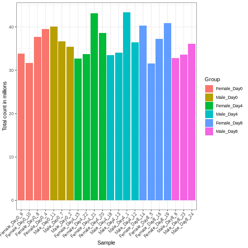
Library size differences
Differences in the total number of reads assigned to genes between samples typically occur for technical reasons. In practice, it means that we can not simply compare a gene’s raw read count directly between samples and conclude that a sample with a higher read count also expresses the gene more strongly - the higher count may be caused by an overall higher number of reads in that sample. In the rest of this section, we will use the term library size to refer to the total number of reads assigned to genes for a sample. First we should compare the library sizes of all samples.
R
# Add in the sum of all counts

se$libSize <-  colSums(assay(se))

# Plot the libSize by using R's native pipe |>
# to extract the colData, turn it into a regular
# data frame then send to ggplot:

colData(se) |>
  as.data.frame() |>
  ggplot(aes(x = Label, y = libSize / 1e6, fill = Group)) +
         geom_bar(stat = "identity") + theme_bw() +
         labs(x = "Sample", y = "Total count in millions") +
         theme(axis.text.x = element_text(angle = 45, hjust = 1, vjust = 1))
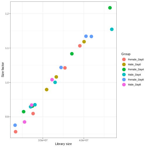
We need to adjust for the differences in library size between samples, to avoid drawing incorrect conclusions. The way this is typically done for RNA-seq data can be described as a two-step procedure. First, we estimate size factors - sample-specific correction factors such that if the raw counts were to be divided by these factors, the resulting values would be more comparable across samples. Next, these size factors are incorporated into the statistical analysis of the data. It is important to pay close attention to how this is done in practice for a given analysis method. Sometimes the division of the counts by the size factors needs to be done explicitly by the analyst. Other times (as we will see for the differential expression analysis) it is important that they are provided separately to the analysis tool, which will then use them appropriately in the statistical model.
With DESeq2, size factors are calculated using the
estimateSizeFactors() function. The size factors estimated
by this function combines an adjustment for differences in library sizes
with an adjustment for differences in the RNA composition of the
samples. The latter is important due to the compositional nature of
RNA-seq data. There is a fixed number of reads to distribute between the
genes, and if a single (or a few) very highly expressed gene consume a
large part of the reads, all other genes will consequently receive very
low counts. We now switch our SummarizedExperiment object
over to a DESeqDataSet as it has the internal structure to
store these size factors. We also need to tell it our main experiment
design, which is sex and time:
R
dds <- DESeq2::DESeqDataSet(se, design = ~ sex + time)
WARNING
Warning in DESeq2::DESeqDataSet(se, design = ~sex + time): some variables in
design formula are characters, converting to factors
R
dds <- estimateSizeFactors(dds)

# Plot the size factors against library size
# and look for any patterns by group:

ggplot(data.frame(libSize = colSums(assay(dds)),
                  sizeFactor = sizeFactors(dds),
                  Group = dds$Group),
       aes(x = libSize, y = sizeFactor, col = Group)) +
    geom_point(size = 5) + theme_bw() +
    labs(x = "Library size", y = "Size factor")
Transform data
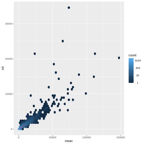
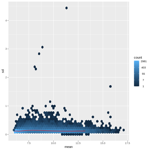
There is a rich literature on methods for exploratory analysis. Most of these work best in situations where the variance of the input data (here, each gene) is relatively independent of the average value. For read count data such as RNA-seq, this is not the case. In fact, the variance increases with the average read count.
R
meanSdPlot(assay(dds), ranks = FALSE)
There are two ways around this: either we develop methods specifically adapted to count data, or we adapt (transform) the count data so that the existing methods are applicable. Both ways have been explored; however, at the moment the second approach is arguably more widely applied in practice. We can transform our data using DESeq2’s variance stabilizing transformation and then verify that it has removed the correlation between average read count and variance.
R
vsd <- DESeq2::vst(dds, blind = TRUE)
meanSdPlot(assay(vsd), ranks = FALSE)
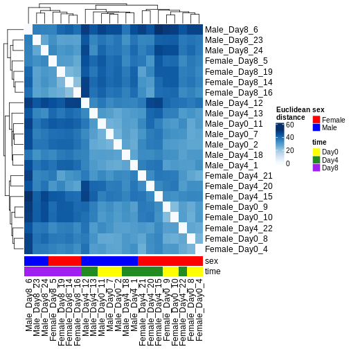
Heatmaps and clustering
There are many ways to cluster samples based on their similarity of expression patterns. One simple way is to calculate Euclidean distances between all pairs of samples (longer distance = more different) and then display the results with both a branching dendrogram and a heatmap to visualize the distances in color. From this, we infer that the Day 8 samples are more similar to each other than the rest of the samples, although Day 4 and Day 0 do not separate distinctly. Instead, males and females reliably separate.
R
dst <- dist(t(assay(vsd)))
colors <- colorRampPalette(brewer.pal(9, "Blues"))(255)
ComplexHeatmap::Heatmap(
    as.matrix(dst),
    col = colors,
    name = "Euclidean\ndistance",
    cluster_rows = hclust(dst),
    cluster_columns = hclust(dst),
    bottom_annotation = columnAnnotation(
        sex = vsd$sex,
        time = vsd$time,
        col = list(sex = c(Female = "red", Male = "blue"),
                   time = c(Day0 = "yellow", Day4 = "forestgreen", Day8 = "purple")))
)
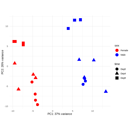
PCA
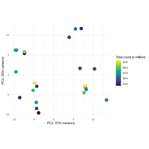
Principal component analysis is a dimensionality reduction method, which projects the samples into a lower-dimensional space. This lower-dimensional representation can be used for visualization, or as the input for other analysis methods. The principal components are defined in such a way that they are orthogonal, and that the projection of the samples into the space they span contains as much variance as possible. It is an unsupervised method in the sense that no external information about the samples (e.g., the treatment condition) is taken into account. In the plot below we represent the samples in a two-dimensional principal component space. For each of the two dimensions, we indicate the fraction of the total variance that is represented by that component. By definition, the first principal component will always represent more of the variance than the subsequent ones. The fraction of explained variance is a measure of how much of the ‘signal’ in the data that is retained when we project the samples from the original, high-dimensional space to the low-dimensional space for visualization.
R
pcaData <- DESeq2::plotPCA(vsd, intgroup = c("sex", "time"),
                           returnData = TRUE)
OUTPUT
using ntop=500 top features by varianceR
percentVar <- round(100 * attr(pcaData, "percentVar"))
ggplot(pcaData, aes(x = PC1, y = PC2)) +
    geom_point(aes(color = sex, shape = time), size = 5) +
    theme_minimal() +
    xlab(paste0("PC1: ", percentVar[1], "% variance")) +
    ylab(paste0("PC2: ", percentVar[2], "% variance")) +
    coord_fixed() +
    scale_color_manual(values = c(Male = "blue", Female = "red"))
Challenge: Discuss the following points with your neighbour
Assume you are mainly interested in expression changes associated with the time after infection (Reminder Day0 -> before infection). What do you need to consider in downstream analysis?
Consider an experimental design where you have multiple samples from the same donor. You are still interested in differences by time and observe the following PCA plot. What does this PCA plot suggest?
OUTPUT
using ntop=500 top features by variance
The major signal in this data (37% variance) is associated with sex. As we are not interested in sex-specific changes over time, we need to adjust for this in downstream analysis (see next episodes) and keep it in mind for further exploratory downstream analysis. A possible way to do so is to remove genes on sex chromosomes.
- A strong donor effect, that needs to be accounted for.
- What does PC1 (37% variance) represent? Looks like 2 donor groups?
- No association of PC1 and PC2 with time –> no or weak transcriptional effect of time --> Check association with higher PCs (e.g., PC3,PC4, ..)
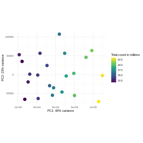
Challenge: Plot the PCA colored by library sizes.
Compare before and after variance stabilizing transformation.
Hint: The DESeq2::plotPCA expect an object of the
class DESeqTransform as input. You can transform a
SummarizedExperiment object using
plotPCA(DESeqTransform(se))
R
pcaDataVst <- DESeq2::plotPCA(vsd, intgroup = c("libSize"),
                              returnData = TRUE)
OUTPUT
using ntop=500 top features by varianceR
percentVar <- round(100 * attr(pcaDataVst, "percentVar"))
ggplot(pcaDataVst, aes(x = PC1, y = PC2)) +
    geom_point(aes(color = libSize / 1e6), size = 5) +
    theme_minimal() +
    xlab(paste0("PC1: ", percentVar[1], "% variance")) +
    ylab(paste0("PC2: ", percentVar[2], "% variance")) +
    coord_fixed() +
    scale_color_continuous("Total count in millions", type = "viridis")
R
pcaDataCts <- DESeq2::plotPCA(DESeqTransform(se), intgroup = c("libSize"),
                              returnData = TRUE)
OUTPUT
using ntop=500 top features by varianceR
percentVar <- round(100 * attr(pcaDataCts, "percentVar"))
ggplot(pcaDataCts, aes(x = PC1, y = PC2)) +
    geom_point(aes(color = libSize / 1e6), size = 5) +
    theme_minimal() +
    xlab(paste0("PC1: ", percentVar[1], "% variance")) +
    ylab(paste0("PC2: ", percentVar[2], "% variance")) +
    coord_fixed() +
    scale_color_continuous("Total count in millions", type = "viridis")
Interactive exploratory data analysis
Often it is useful to look at QC plots in an interactive way to directly explore different experimental factors or get insides from someone without coding experience. Useful tools for interactive exploratory data analysis for RNA-seq are Glimma and iSEE
Challenge: Interactively explore our data using iSEE
R
## Convert DESeqDataSet object to a SingleCellExperiment object, in order to
## be able to store the PCA representation
sce <- as(dds, "SingleCellExperiment")

## Add PCA to the 'reducedDim' slot
stopifnot(rownames(pcaData) == colnames(sce))
reducedDim(sce, "PCA") <- as.matrix(pcaData[, c("PC1", "PC2")])

## Add variance-stabilized data as a new assay
stopifnot(colnames(vsd) == colnames(sce))
assay(sce, "vsd") <- assay(vsd)

app <- iSEE(sce)
shiny::runApp(app)
Session info
R
sessionInfo()
OUTPUT
R version 4.5.2 (2025-10-31)
Platform: x86_64-pc-linux-gnu
Running under: Ubuntu 22.04.5 LTS

Matrix products: default
BLAS:   /usr/lib/x86_64-linux-gnu/blas/libblas.so.3.10.0
LAPACK: /usr/lib/x86_64-linux-gnu/lapack/liblapack.so.3.10.0  LAPACK version 3.10.0

locale:
 [1] LC_CTYPE=C.UTF-8       LC_NUMERIC=C           LC_TIME=C.UTF-8
 [4] LC_COLLATE=C.UTF-8     LC_MONETARY=C.UTF-8    LC_MESSAGES=C.UTF-8
 [7] LC_PAPER=C.UTF-8       LC_NAME=C              LC_ADDRESS=C
[10] LC_TELEPHONE=C         LC_MEASUREMENT=C.UTF-8 LC_IDENTIFICATION=C

time zone: UTC
tzcode source: system (glibc)

attached base packages:
[1] grid      stats4    stats     graphics  grDevices utils     datasets
[8] methods   base

other attached packages:
 [1] iSEE_2.20.0                 SingleCellExperiment_1.30.1
 [3] hexbin_1.28.5               RColorBrewer_1.1-3
 [5] ComplexHeatmap_2.24.1       ggplot2_3.5.2
 [7] vsn_3.76.0                  DESeq2_1.48.1
 [9] SummarizedExperiment_1.38.1 Biobase_2.68.0
[11] MatrixGenerics_1.20.0       matrixStats_1.5.0
[13] GenomicRanges_1.60.0        GenomeInfoDb_1.44.1
[15] IRanges_2.42.0              S4Vectors_0.46.0
[17] BiocGenerics_0.54.0         generics_0.1.4

loaded via a namespace (and not attached):
 [1] rlang_1.1.6             magrittr_2.0.4          shinydashboard_0.7.3
 [4] clue_0.3-66             GetoptLong_1.0.5        pegboard_0.7.9
 [7] compiler_4.5.2          mgcv_1.9-3              png_0.1-8
[10] callr_3.7.6             vctrs_0.6.5             pkgconfig_2.0.3
[13] shape_1.4.6.1           crayon_1.5.3            fastmap_1.2.0
[16] XVector_0.48.0          labeling_0.4.3          promises_1.3.3
[19] shinyAce_0.4.4          UCSC.utils_1.4.0        ps_1.9.1
[22] preprocessCore_1.70.0   purrr_1.2.0             xfun_0.52
[25] cachem_1.1.0            jsonlite_2.0.0          listviewer_4.0.0
[28] later_1.4.2             DelayedArray_0.34.1     BiocParallel_1.42.1
[31] parallel_4.5.2          cluster_2.1.8.1         R6_2.6.1
[34] bslib_0.9.0             limma_3.64.3            jquerylib_0.1.4
[37] Rcpp_1.1.0              assertthat_0.2.1        iterators_1.0.14
[40] knitr_1.50              splines_4.5.2           igraph_2.1.4
[43] httpuv_1.6.16           Matrix_1.7-3            tidyselect_1.2.1
[46] abind_1.4-8             yaml_2.3.10             doParallel_1.0.17
[49] codetools_0.2-20        affy_1.86.0             miniUI_0.1.2
[52] processx_3.8.6          lattice_0.22-7          tibble_3.3.0
[55] shiny_1.11.1            withr_3.0.2             evaluate_1.0.4
[58] sandpaper_0.17.2.9000   xml2_1.4.1              circlize_0.4.16
[61] pillar_1.11.0           affyio_1.78.0           BiocManager_1.30.26
[64] renv_1.1.5              DT_0.33                 foreach_1.5.2
[67] shinyjs_2.1.0           scales_1.4.0            xtable_1.8-4
[70] glue_1.8.0              tools_4.5.2             colourpicker_1.3.0
[73] locfit_1.5-9.12         colorspace_2.1-1        nlme_3.1-168
[76] GenomeInfoDbData_1.2.14 tinkr_0.3.0             vipor_0.4.7
[79] cli_3.6.5               viridisLite_0.4.2       S4Arrays_1.8.1
[82] dplyr_1.1.4             gtable_0.3.6            rintrojs_0.3.4
[85] sass_0.4.10             digest_0.6.37           SparseArray_1.8.1
[88] ggrepel_0.9.6           rjson_0.2.23            htmlwidgets_1.6.4
[91] farver_2.1.2            htmltools_0.5.8.1       lifecycle_1.0.4
[94] shinyWidgets_0.9.0      httr_1.4.7              GlobalOptions_0.1.2
[97] statmod_1.5.0 mime_0.13 - Exploratory analysis is essential for quality control and to detect potential problems with a data set.
- Different classes of exploratory analysis methods expect differently preprocessed data. The most commonly used methods expect counts to be normalized and log-transformed (or similar- more sensitive/sophisticated), to be closer to homoskedastic. Other methods work directly on the raw counts.
Content from Differential expression analysis
Last updated on 2025-11-11 | Edit this page
Estimated time 105 minutes
Overview
Questions
- What are the steps performed in a typical differential expression analysis?
- How does one interpret the output of DESeq2?
Objectives
- Explain the steps involved in a differential expression analysis.
- Explain how to perform these steps in R, using DESeq2.
Differential expression inference
A major goal of RNA-seq data analysis is the quantification and statistical inference of systematic changes between experimental groups or conditions (e.g., treatment vs. control, timepoints, tissues). This is typically performed by identifying genes with differential expression pattern using between- and within-condition variability and thus requires biological replicates (multiple sample of the same condition). Multiple software packages exist to perform differential expression analysis. Comparative studies have shown some concordance of differentially expressed (DE) genes, but also variability between tools with no tool consistently outperforming all others (see Soneson and Delorenzi, 2013). In the following we will explain and conduct differential expression analysis using the DESeq2 software package. The edgeR package implements similar methods following the same main assumptions about count data. Both packages show a general good and stable performance with comparable results.
The DESeqDataSet
To run DESeq2 we need to represent our count data as
object of the DESeqDataSet class. The
DESeqDataSet is an extension of the
SummarizedExperiment class (see section Importing and annotating quantified data
into R ) that stores a design formula in addition to the
count assay(s) and feature (here gene) and sample metadata. The
design formula expresses the variables which will be used in
modeling. These are typically the variable of interest (group variable)
and other variables you want to account for (e.g., batch effect
variables). A detailed explanation of design formulas and
related design matrices will follow in the section about extra exploration of design matrices.
Objects of the DESeqDataSet class can be build from count
matrices, SummarizedExperiment
objects, transcript
abundance files or htseq
count files.
Load packages
R
suppressPackageStartupMessages({
    library(SummarizedExperiment)
    library(DESeq2)
    library(ggplot2)
    library(ExploreModelMatrix)
    library(cowplot)
    library(ComplexHeatmap)
    library(apeglm)
})
Load data
Let’s load in our SummarizedExperiment object again. In
the last episode for quality control exploration, we removed ~35% genes
that had 5 or fewer counts because they had too little information in
them. For DESeq2 statistical analysis, we do not technically have to
remove these genes because by default it will do some independent
filtering, but it can reduce the memory size of the
DESeqDataSet object resulting in faster computation. Plus,
we do not want these genes cluttering up some of the visualizations.
R
se <- readRDS("data/GSE96870_se.rds")
se <- se[rowSums(assay(se, "counts")) > 5, ]
Create DESeqDataSet
The design matrix we will use in this example is
~ sex + time. This will allow us test the difference
between males and females (averaged over time point) and the difference
between day 0, 4 and 8 (averaged over males and females). If we wanted
to test other comparisons (e.g., Female.Day8 vs. Female.Day0 and also
Male.Day8 vs. Male.Day0) we could use a different design matrix to more
easily extract those pairwise comparisons.
R
dds <- DESeq2::DESeqDataSet(se,
                            design = ~ sex + time)
WARNING
Warning in DESeq2::DESeqDataSet(se, design = ~sex + time): some variables in
design formula are characters, converting to factorsThe function to generate a DESeqDataSet needs to be
adapted depending on the input type, e.g,
R
#From SummarizedExperiment object
ddsSE <- DESeqDataSet(se, design = ~ sex + time)

#From count matrix
dds <- DESeqDataSetFromMatrix(countData = assays(se)$counts,
                              colData = colData(se),
                              design = ~ sex + time)
Normalization
DESeq2 and edgeR make the following
assumptions:
- most genes are not differentially expressed
- the probability of a read mapping to a specific gene is the same for all samples within the same group
As shown in the previous section
on exploratory data analysis the total counts of a sample (even from the
same condition) depends on the library size (total number of reads
sequenced). To compare the variability of counts from a specific gene
between and within groups we first need to account for library sizes and
compositional effects. Recall the estimateSizeFactors()
function from the previous section:
R
dds <- estimateSizeFactors(dds)
DESeq2 uses the “Relative Log Expression” (RLE) method to calculate sample-wise size factors tĥat account for read depth and library composition. edgeR uses the “Trimmed Mean of M-Values” (TMM) method to account for library size differences and compositional effects. edgeR’s normalization factors and DESeq2’s size factors yield similar results, but are not equivalent theoretical parameters.
Statistical modeling
DESeq2 and edgeR model RNA-seq counts as
negative binomial distribution to account for a limited
number of replicates per group, a mean-variance dependency (see exploratory data analysis) and a
skewed count distribution.
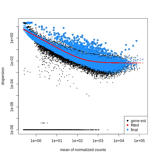
Dispersion
The within-group variance of the counts for a gene following a negative binomial distribution with mean \(\mu\) can be modeled as:
\(var = \mu + \theta \mu^2\)
\(\theta\) represents the
gene-specific dispersion, a measure of variability or
spread in the data. As a second step, we need to estimate gene-wise
dispersions to get the expected within-group variance and test for group
differences. Good dispersion estimates are challenging with a few
samples per group only. Thus, information from genes with similar
expression pattern are “borrowed”. Gene-wise dispersion estimates are
shrinked towards center values of the observed distribution of
dispersions. With DESeq2 we can get dispersion estimates
using the estimateDispersions() function. We can visualize
the effect of shrinkage using plotDispEsts():
R
dds <- estimateDispersions(dds)
OUTPUT
gene-wise dispersion estimatesOUTPUT
mean-dispersion relationshipOUTPUT
final dispersion estimatesR
plotDispEsts(dds)
Testing
We can use the nbinomWaldTest()function of
DESeq2 to fit a generalized linear model (GLM) and
compute log2 fold changes (synonymous with “GLM coefficients”,
“beta coefficients” or “effect size”) corresponding to the variables of
the design matrix. The design matrix is directly
related to the design formula and automatically derived from
it. Assume a design formula with one variable (~ treatment)
and two factor levels (treatment and control). The mean expression \(\mu_{j}\) of a specific gene in sample
\(j\) will be modeled as following:
\(log(μ_j) = β_0 + x_j β_T\),
with \(β_T\) corresponding to the log2 fold change of the treatment groups, \(x_j\) = 1, if \(j\) belongs to the treatment group and \(x_j\) = 0, if \(j\) belongs to the control group.
Finally, the estimated log2 fold changes are scaled by their standard error and tested for being significantly different from 0 using the Wald test.
R
dds <- nbinomWaldTest(dds)
Note
Standard differential expression analysis as performed above is
wrapped into a single function, DESeq(). Running the first
code chunk is equivalent to running the second one:
R
dds <- DESeq(dds)
R
dds <- estimateSizeFactors(dds)
dds <- estimateDispersions(dds)
dds <- nbinomWaldTest(dds)
Explore results for specific contrasts
The results() function can be used to extract gene-wise
test statistics, such as log2 fold changes and (adjusted) p-values. The
comparison of interest can be defined using contrasts, which are linear
combinations of the model coefficients (equivalent to combinations of
columns within the design matrix) and thus directly related to
the design formula. A detailed explanation of design matrices and how to
use them to specify different contrasts of interest can be found in the
section on the exploration of design
matrices. In the results() function a contrast can be
represented by the variable of interest (reference variable) and the
related level to compare using the contrast argument. By
default the reference variable will be the last
variable of the design formula, the reference level
will be the first factor level and the last level will be used
for comparison. You can also explicitly specify a contrast by the
name argument of the results() function. Names
of all available contrasts can be accessed using
resultsNames().
Challenge
What will be the default contrast, reference
level and “last level” for comparisons when
running results(dds) for the example used in this
lesson?
Hint: Check the design formula used to build the object.
In the lesson example the last variable of the design formula is
time. The reference level (first in
alphabetical order) is Day0 and the last
level is Day8
R
levels(dds$time)
OUTPUT
[1] "Day0" "Day4" "Day8"No worries, if you had difficulties to identify the default contrast
the output of the results() function explicitly states the
contrast it is referring to (see below)!
To explore the output of the results() function we can
use the summary() function and order results by
significance (p-value). Here we assume that we are interested in changes
over time (“variable of interest”), more specifically genes
with differential expression between Day0 (“reference
level”) and Day8 (“level to compare”). The model we used
included the sex variable (see above). Thus our results
will be “corrected” for sex-related differences.
R
## Day 8 vs Day 0
resTime <- results(dds, contrast = c("time", "Day8", "Day0"))
summary(resTime)
OUTPUT
out of 27430 with nonzero total read count
adjusted p-value < 0.1
LFC > 0 (up)       : 4472, 16%
LFC < 0 (down)     : 4282, 16%
outliers [1]       : 10, 0.036%
low counts [2]     : 3723, 14%
(mean count < 1)
[1] see 'cooksCutoff' argument of ?results
[2] see 'independentFiltering' argument of ?results
R
# View(resTime)
head(resTime[order(resTime$pvalue), ])
OUTPUT
log2 fold change (MLE): time Day8 vs Day0
Wald test p-value: time Day8 vs Day0
DataFrame with 6 rows and 6 columns
               baseMean log2FoldChange     lfcSE      stat      pvalue
              <numeric>      <numeric> <numeric> <numeric>   <numeric>
Asl             701.343       1.117332 0.0594128   18.8062 6.71212e-79
Apod          18765.146       1.446981 0.0805056   17.9737 3.13229e-72
Cyp2d22        2550.480       0.910202 0.0556002   16.3705 3.10712e-60
Klk6            546.503      -1.671897 0.1057395  -15.8115 2.59339e-56
Fcrls           184.235      -1.947016 0.1277235  -15.2440 1.80488e-52
A330076C08Rik   107.250      -1.749957 0.1155125  -15.1495 7.63434e-52
                     padj
                <numeric>
Asl           1.59057e-74
Apod          3.71130e-68
Cyp2d22       2.45431e-56
Klk6          1.53639e-52
Fcrls         8.55406e-49
A330076C08Rik 3.01518e-48Both of the below ways of specifying the contrast are essentially
equivalent. The name parameter can be accessed using
resultsNames().
R
resTime <- results(dds, contrast = c("time", "Day8", "Day0"))
resTime <- results(dds, name = "time_Day8_vs_Day0")
Challenge
Explore the DE genes between males and females independent of time.
Hint: You don’t need to fit the GLM again. Use
resultsNames() to get the correct contrast.
R
## Male vs Female
resSex <- results(dds, contrast = c("sex", "Male", "Female"))
summary(resSex)
OUTPUT
out of 27430 with nonzero total read count
adjusted p-value < 0.1
LFC > 0 (up)       : 51, 0.19%
LFC < 0 (down)     : 70, 0.26%
outliers [1]       : 10, 0.036%
low counts [2]     : 8504, 31%
(mean count < 6)
[1] see 'cooksCutoff' argument of ?results
[2] see 'independentFiltering' argument of ?results
R
head(resSex[order(resSex$pvalue), ])
OUTPUT
log2 fold change (MLE): sex Male vs Female
Wald test p-value: sex Male vs Female
DataFrame with 6 rows and 6 columns
               baseMean log2FoldChange     lfcSE      stat       pvalue
              <numeric>      <numeric> <numeric> <numeric>    <numeric>
Xist         22603.0359      -11.60429  0.336282  -34.5076 6.16852e-261
Ddx3y         2072.9436       11.87241  0.397493   29.8683 5.08722e-196
Eif2s3y       1410.8750       12.62513  0.565194   22.3377 1.58997e-110
Kdm5d          692.1672       12.55386  0.593607   21.1484  2.85293e-99
Uty            667.4375       12.01728  0.593573   20.2457  3.87772e-91
LOC105243748    52.9669        9.08325  0.597575   15.2002  3.52699e-52
                     padj
                <numeric>
Xist         1.16684e-256
Ddx3y        4.81149e-192
Eif2s3y      1.00253e-106
Kdm5d         1.34915e-95
Uty           1.46702e-87
LOC105243748 1.11194e-48Multiple testing correction
Due to the high number of tests (one per gene) our DE results will contain a substantial number of false positives. For example, if we tested 20,000 genes at a threshold of \(\alpha = 0.05\) we would expect 1,000 significant DE genes with no differential expression.
To account for this expected high number of false positives, we can
correct our results for multiple testing. By default
DESeq2 uses the Benjamini-Hochberg
procedure to calculate adjusted p-values (padj) for
DE results.
Independent Filtering and log-fold shrinkage
We can visualize the results in many ways. A good check is to explore
the relationship between log2fold changes, significant DE
genes and the genes mean count. DESeq2
provides a useful function to do so, plotMA().
R
plotMA(resTime)
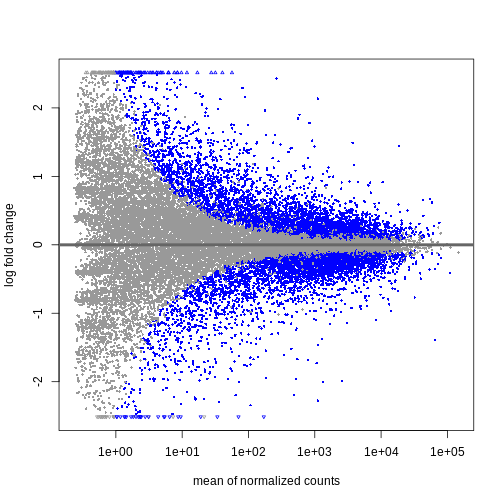
We can see that genes with a low mean count tend to have larger log fold changes. This is caused by counts from lowly expressed genes tending to be very noisy. We can shrink the log fold changes of these genes with low mean and high dispersion, as they contain little information.
R
resTimeLfc <- lfcShrink(dds, coef = "time_Day8_vs_Day0", res = resTime)
OUTPUT
using 'apeglm' for LFC shrinkage. If used in published research, please cite:
    Zhu, A., Ibrahim, J.G., Love, M.I. (2018) Heavy-tailed prior distributions for
    sequence count data: removing the noise and preserving large differences.
    Bioinformatics. https://doi.org/10.1093/bioinformatics/bty895
R
plotMA(resTimeLfc)
Shrinkage of log fold changes is useful for visualization and ranking
of genes, but for result exploration typically the
independentFiltering argument is used to remove lowly
expressed genes.
Challenge
By default independentFiltering is set to
TRUE. What happens without filtering lowly expressed genes?
Use the summary() function to compare the results. Most of
the lowly expressed genes are not significantly differential expressed
(blue in the above MA plots). What could cause the difference in the
results then?
R
resTimeNotFiltered <- results(dds,
                              contrast = c("time", "Day8", "Day0"),
                              independentFiltering = FALSE)
summary(resTime)
OUTPUT
out of 27430 with nonzero total read count
adjusted p-value < 0.1
LFC > 0 (up)       : 4472, 16%
LFC < 0 (down)     : 4282, 16%
outliers [1]       : 10, 0.036%
low counts [2]     : 3723, 14%
(mean count < 1)
[1] see 'cooksCutoff' argument of ?results
[2] see 'independentFiltering' argument of ?results
R
summary(resTimeNotFiltered)
OUTPUT
out of 27430 with nonzero total read count
adjusted p-value < 0.1
LFC > 0 (up)       : 4324, 16%
LFC < 0 (down)     : 4129, 15%
outliers [1]       : 10, 0.036%
low counts [2]     : 0, 0%
(mean count < 0)
[1] see 'cooksCutoff' argument of ?results
[2] see 'independentFiltering' argument of ?results
Genes with very low counts are not likely to see significant differences typically due to high dispersion. Filtering of lowly expressed genes thus increased detection power at the same experiment-wide false positive rate.
Visualize selected set of genes
The amount of DE genes can be overwhelming and a ranked list of genes can still be hard to interpret with regards to an experimental question. Visualizing gene expression can help to detect expression pattern or group of genes with related functions. We will perform systematic detection of over represented groups of genes in a later section. Before this visualization can already help us to get a good intuition about what to expect.
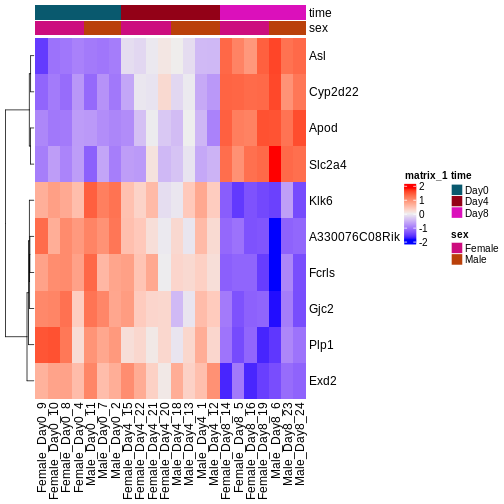
We will use transformed data (see exploratory data analysis) and the top differentially expressed genes for visualization. A heatmap can reveal expression pattern across sample groups (columns) and automatically orders genes (rows) according to their similarity.
R
# Transform counts
vsd <- vst(dds, blind = TRUE)

# Get top DE genes
genes <- resTime[order(resTime$pvalue), ] |>
         head(10) |>
         rownames()
heatmapData <- assay(vsd)[genes, ]

# Scale counts for visualization
heatmapData <- t(scale(t(heatmapData)))

# Add annotation
heatmapColAnnot <- data.frame(colData(vsd)[, c("time", "sex")])
heatmapColAnnot <- HeatmapAnnotation(df = heatmapColAnnot)

# Plot as heatmap
ComplexHeatmap::Heatmap(heatmapData,
                        top_annotation = heatmapColAnnot,
                        cluster_rows = TRUE, cluster_columns = FALSE)
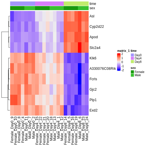
Challenge
Check the heatmap and top DE genes. Do you find something expected/unexpected in terms of change across all 3 time points?
Output results
We may want to to output our results out of R to have a stand-alone
file. The format of resTime only has the gene symbols as
rownames, so let us join the gene annotation information, and then write
out as .csv file:
R
head(as.data.frame(resTime))
head(as.data.frame(rowRanges(se)))

temp <- cbind(as.data.frame(rowRanges(se)),
              as.data.frame(resTime))

write.csv(temp, file = "output/Day8vsDay0.csv")
- With DESeq2, the main steps of a differential expression analysis (size factor estimation, dispersion estimation, calculation of test statistics) are wrapped in a single function: DESeq().
- Independent filtering of lowly expressed genes is often beneficial.
Content from Extra exploration of design matrices
Last updated on 2025-11-11 | Edit this page
Estimated time 60 minutes
Overview
Questions
- How can one translate biological questions and comparisons to statistical terms suitable for use with RNA-seq analysis packages?
Objectives
- Explain the formula notation and design matrices.
- Explore different designs and learn how to interpret coefficients.
Loading required packages and reading data
We start by loading a few packages that will be needed in this episode. In particular, the ExploreModelMatrix package provides resources for exploring design matrices in a graphical fashion, for easier interpretation.
R
suppressPackageStartupMessages({
    library(SummarizedExperiment)
    library(ExploreModelMatrix)
    library(dplyr)
    library(DESeq2)
})
Next, we read the metadata table for our data set. Because we want to explore many different design matrices, we will read in the 4th file we downloaded but haven’t used yet: that for both Cerebellum and Spinal Cord samples (45 samples total). As seen in previous episodes, the metadata contains information about the age, sex, infection status, time of measurement and tissue of the collected samples. Note that Day0 always corresponds to non-infected samples, and that infected samples are collected on days 4 and 8. Moreover, all mice have the same age (8 weeks). Hence, in the first part of this episode we consider only the sex, tissue and time variables further.
R
meta <- read.csv("data/GSE96870_coldata_all.csv", row.names = 1)
# Here, for brevity we only print the first rows of the data.frame
head(meta)
OUTPUT
                     title geo_accession     organism     age    sex
GSM2545336 CNS_RNA-seq_10C    GSM2545336 Mus musculus 8 weeks Female
GSM2545337 CNS_RNA-seq_11C    GSM2545337 Mus musculus 8 weeks Female
GSM2545338 CNS_RNA-seq_12C    GSM2545338 Mus musculus 8 weeks Female
GSM2545339 CNS_RNA-seq_13C    GSM2545339 Mus musculus 8 weeks Female
GSM2545340 CNS_RNA-seq_14C    GSM2545340 Mus musculus 8 weeks   Male
GSM2545341 CNS_RNA-seq_17C    GSM2545341 Mus musculus 8 weeks   Male
             infection  strain time     tissue mouse
GSM2545336  InfluenzaA C57BL/6 Day8 Cerebellum    14
GSM2545337 NonInfected C57BL/6 Day0 Cerebellum     9
GSM2545338 NonInfected C57BL/6 Day0 Cerebellum    10
GSM2545339  InfluenzaA C57BL/6 Day4 Cerebellum    15
GSM2545340  InfluenzaA C57BL/6 Day4 Cerebellum    18
GSM2545341  InfluenzaA C57BL/6 Day8 Cerebellum     6
R
table(meta$time, meta$infection)
OUTPUT
       InfluenzaA NonInfected
  Day0          0          15
  Day4         16           0
  Day8         14           0
R
table(meta$age)
OUTPUT
8 weeks
     45
We can start by visualizing the number of observations for each combination of the three predictor variables.
R
vd <- VisualizeDesign(sampleData = meta,
                      designFormula = ~ tissue + time + sex)
vd$cooccurrenceplots
OUTPUT
$`tissue = Cerebellum`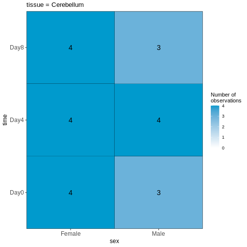
OUTPUT
$`tissue = Spinalcord`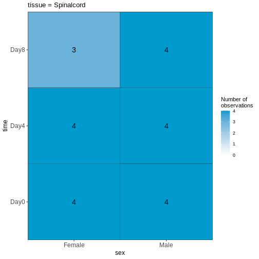
Challenge
Based on this visualization, would you say that the data set is balanced, or are there combinations of predictor variables that are severely over- or underrepresented?
Compare males and females, non-infected spinal cord
Next, we will set up our first design matrix. Here, we will focus on
the uninfected (Day0) spinal cord samples, and our aim is to compare the
male and female mice. Thus, we first subset the metadata to only the
samples of interest, and next set up and visualize the design matrix
with a single predictor variable (sex). By defining the design formula
as ~ sex, we tell R to include an intercept in the design.
This intercept will represent the ‘baseline’ level of the predictor
variable, which in this case is selected to be the Female mice. If not
explicitly specified, R will order the values of the predictor in
alphabetical order and select the first one as the reference or baseline
level.
R
## Subset metadata
meta_noninf_spc <- meta %>% filter(time == "Day0" &
                                       tissue == "Spinalcord")
meta_noninf_spc
OUTPUT
                     title geo_accession     organism     age    sex
GSM2545356 CNS_RNA-seq_574    GSM2545356 Mus musculus 8 weeks   Male
GSM2545357 CNS_RNA-seq_575    GSM2545357 Mus musculus 8 weeks   Male
GSM2545358 CNS_RNA-seq_583    GSM2545358 Mus musculus 8 weeks Female
GSM2545361 CNS_RNA-seq_590    GSM2545361 Mus musculus 8 weeks   Male
GSM2545364 CNS_RNA-seq_709    GSM2545364 Mus musculus 8 weeks Female
GSM2545365 CNS_RNA-seq_710    GSM2545365 Mus musculus 8 weeks Female
GSM2545366 CNS_RNA-seq_711    GSM2545366 Mus musculus 8 weeks Female
GSM2545367 CNS_RNA-seq_713    GSM2545367 Mus musculus 8 weeks   Male
             infection  strain time     tissue mouse
GSM2545356 NonInfected C57BL/6 Day0 Spinalcord     2
GSM2545357 NonInfected C57BL/6 Day0 Spinalcord     3
GSM2545358 NonInfected C57BL/6 Day0 Spinalcord     4
GSM2545361 NonInfected C57BL/6 Day0 Spinalcord     7
GSM2545364 NonInfected C57BL/6 Day0 Spinalcord     8
GSM2545365 NonInfected C57BL/6 Day0 Spinalcord     9
GSM2545366 NonInfected C57BL/6 Day0 Spinalcord    10
GSM2545367 NonInfected C57BL/6 Day0 Spinalcord    11
R
## Use ExploreModelMatrix to create a design matrix and visualizations, given
## the desired design formula.
vd <- VisualizeDesign(sampleData = meta_noninf_spc,
                      designFormula = ~ sex)
vd$designmatrix
OUTPUT
           (Intercept) sexMale
GSM2545356           1       1
GSM2545357           1       1
GSM2545358           1       0
GSM2545361           1       1
GSM2545364           1       0
GSM2545365           1       0
GSM2545366           1       0
GSM2545367           1       1
R
vd$plotlist
OUTPUT
[[1]]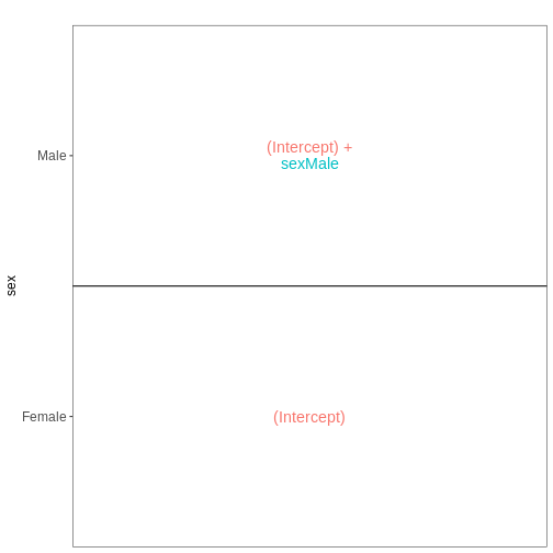
R
## Note that we can also generate the design matrix like this
model.matrix(~ sex, data = meta_noninf_spc)
OUTPUT
           (Intercept) sexMale
GSM2545356           1       1
GSM2545357           1       1
GSM2545358           1       0
GSM2545361           1       1
GSM2545364           1       0
GSM2545365           1       0
GSM2545366           1       0
GSM2545367           1       1
attr(,"assign")
[1] 0 1
attr(,"contrasts")
attr(,"contrasts")$sex
[1] "contr.treatment"Challenge
With this design, what is the interpretation of the
sexMale coefficient?
Challenge
Set up the design formula to compare male and female spinal cord samples from Day0 as above, but instruct R to not include an intercept in the model. How does this change the interpretation of the coefficients? What contrast would have to be specified to compare the mean expression of a gene between male and female mice?
R
meta_noninf_spc <- meta %>% filter(time == "Day0" &
                                       tissue == "Spinalcord")
meta_noninf_spc
OUTPUT
                     title geo_accession     organism     age    sex
GSM2545356 CNS_RNA-seq_574    GSM2545356 Mus musculus 8 weeks   Male
GSM2545357 CNS_RNA-seq_575    GSM2545357 Mus musculus 8 weeks   Male
GSM2545358 CNS_RNA-seq_583    GSM2545358 Mus musculus 8 weeks Female
GSM2545361 CNS_RNA-seq_590    GSM2545361 Mus musculus 8 weeks   Male
GSM2545364 CNS_RNA-seq_709    GSM2545364 Mus musculus 8 weeks Female
GSM2545365 CNS_RNA-seq_710    GSM2545365 Mus musculus 8 weeks Female
GSM2545366 CNS_RNA-seq_711    GSM2545366 Mus musculus 8 weeks Female
GSM2545367 CNS_RNA-seq_713    GSM2545367 Mus musculus 8 weeks   Male
             infection  strain time     tissue mouse
GSM2545356 NonInfected C57BL/6 Day0 Spinalcord     2
GSM2545357 NonInfected C57BL/6 Day0 Spinalcord     3
GSM2545358 NonInfected C57BL/6 Day0 Spinalcord     4
GSM2545361 NonInfected C57BL/6 Day0 Spinalcord     7
GSM2545364 NonInfected C57BL/6 Day0 Spinalcord     8
GSM2545365 NonInfected C57BL/6 Day0 Spinalcord     9
GSM2545366 NonInfected C57BL/6 Day0 Spinalcord    10
GSM2545367 NonInfected C57BL/6 Day0 Spinalcord    11
R
vd <- VisualizeDesign(sampleData = meta_noninf_spc,
                      designFormula = ~ 0 + sex)
vd$designmatrix
OUTPUT
           sexFemale sexMale
GSM2545356         0       1
GSM2545357         0       1
GSM2545358         1       0
GSM2545361         0       1
GSM2545364         1       0
GSM2545365         1       0
GSM2545366         1       0
GSM2545367         0       1
R
vd$plotlist
OUTPUT
[[1]]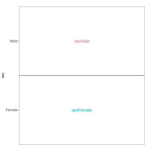
Challenge
Set up the design formula to compare the three time points (Day0,
Day4, Day8) in the male spinal cord samples, and visualize it using
ExploreModelMatrix.
R
meta_male_spc <- meta %>% filter(sex == "Male" & tissue == "Spinalcord")
meta_male_spc
OUTPUT
                     title geo_accession     organism     age  sex   infection
GSM2545355 CNS_RNA-seq_571    GSM2545355 Mus musculus 8 weeks Male  InfluenzaA
GSM2545356 CNS_RNA-seq_574    GSM2545356 Mus musculus 8 weeks Male NonInfected
GSM2545357 CNS_RNA-seq_575    GSM2545357 Mus musculus 8 weeks Male NonInfected
GSM2545360 CNS_RNA-seq_589    GSM2545360 Mus musculus 8 weeks Male  InfluenzaA
GSM2545361 CNS_RNA-seq_590    GSM2545361 Mus musculus 8 weeks Male NonInfected
GSM2545367 CNS_RNA-seq_713    GSM2545367 Mus musculus 8 weeks Male NonInfected
GSM2545368 CNS_RNA-seq_728    GSM2545368 Mus musculus 8 weeks Male  InfluenzaA
GSM2545369 CNS_RNA-seq_729    GSM2545369 Mus musculus 8 weeks Male  InfluenzaA
GSM2545372 CNS_RNA-seq_733    GSM2545372 Mus musculus 8 weeks Male  InfluenzaA
GSM2545373 CNS_RNA-seq_735    GSM2545373 Mus musculus 8 weeks Male  InfluenzaA
GSM2545378 CNS_RNA-seq_742    GSM2545378 Mus musculus 8 weeks Male  InfluenzaA
GSM2545379 CNS_RNA-seq_743    GSM2545379 Mus musculus 8 weeks Male  InfluenzaA
            strain time     tissue mouse
GSM2545355 C57BL/6 Day4 Spinalcord     1
GSM2545356 C57BL/6 Day0 Spinalcord     2
GSM2545357 C57BL/6 Day0 Spinalcord     3
GSM2545360 C57BL/6 Day8 Spinalcord     6
GSM2545361 C57BL/6 Day0 Spinalcord     7
GSM2545367 C57BL/6 Day0 Spinalcord    11
GSM2545368 C57BL/6 Day4 Spinalcord    12
GSM2545369 C57BL/6 Day4 Spinalcord    13
GSM2545372 C57BL/6 Day8 Spinalcord    17
GSM2545373 C57BL/6 Day4 Spinalcord    18
GSM2545378 C57BL/6 Day8 Spinalcord    23
GSM2545379 C57BL/6 Day8 Spinalcord    24
R
vd <- VisualizeDesign(sampleData = meta_male_spc, designFormula = ~ time)
vd$designmatrix
OUTPUT
           (Intercept) timeDay4 timeDay8
GSM2545355           1        1        0
GSM2545356           1        0        0
GSM2545357           1        0        0
GSM2545360           1        0        1
GSM2545361           1        0        0
GSM2545367           1        0        0
GSM2545368           1        1        0
GSM2545369           1        1        0
GSM2545372           1        0        1
GSM2545373           1        1        0
GSM2545378           1        0        1
GSM2545379           1        0        1
R
vd$plotlist
OUTPUT
[[1]]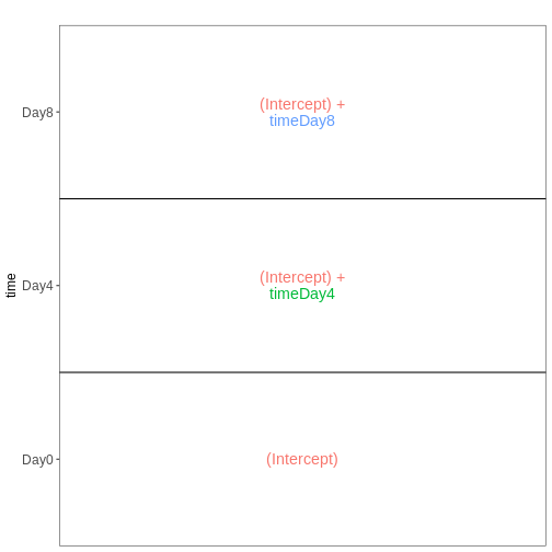
Factorial design without interactions
Next, we again consider only non-infected mice, but fit a model incorporating both sex and tissue as predictors. We assume that the tissue differences are the same for both male and female mice, and consequently fit an additive model, without interaction terms.
R
meta_noninf <- meta %>% filter(time == "Day0")
meta_noninf
OUTPUT
                     title geo_accession     organism     age    sex
GSM2545337 CNS_RNA-seq_11C    GSM2545337 Mus musculus 8 weeks Female
GSM2545338 CNS_RNA-seq_12C    GSM2545338 Mus musculus 8 weeks Female
GSM2545343 CNS_RNA-seq_20C    GSM2545343 Mus musculus 8 weeks   Male
GSM2545348 CNS_RNA-seq_27C    GSM2545348 Mus musculus 8 weeks Female
GSM2545349 CNS_RNA-seq_28C    GSM2545349 Mus musculus 8 weeks   Male
GSM2545353  CNS_RNA-seq_3C    GSM2545353 Mus musculus 8 weeks Female
GSM2545354  CNS_RNA-seq_4C    GSM2545354 Mus musculus 8 weeks   Male
GSM2545356 CNS_RNA-seq_574    GSM2545356 Mus musculus 8 weeks   Male
GSM2545357 CNS_RNA-seq_575    GSM2545357 Mus musculus 8 weeks   Male
GSM2545358 CNS_RNA-seq_583    GSM2545358 Mus musculus 8 weeks Female
GSM2545361 CNS_RNA-seq_590    GSM2545361 Mus musculus 8 weeks   Male
GSM2545364 CNS_RNA-seq_709    GSM2545364 Mus musculus 8 weeks Female
GSM2545365 CNS_RNA-seq_710    GSM2545365 Mus musculus 8 weeks Female
GSM2545366 CNS_RNA-seq_711    GSM2545366 Mus musculus 8 weeks Female
GSM2545367 CNS_RNA-seq_713    GSM2545367 Mus musculus 8 weeks   Male
             infection  strain time     tissue mouse
GSM2545337 NonInfected C57BL/6 Day0 Cerebellum     9
GSM2545338 NonInfected C57BL/6 Day0 Cerebellum    10
GSM2545343 NonInfected C57BL/6 Day0 Cerebellum    11
GSM2545348 NonInfected C57BL/6 Day0 Cerebellum     8
GSM2545349 NonInfected C57BL/6 Day0 Cerebellum     7
GSM2545353 NonInfected C57BL/6 Day0 Cerebellum     4
GSM2545354 NonInfected C57BL/6 Day0 Cerebellum     2
GSM2545356 NonInfected C57BL/6 Day0 Spinalcord     2
GSM2545357 NonInfected C57BL/6 Day0 Spinalcord     3
GSM2545358 NonInfected C57BL/6 Day0 Spinalcord     4
GSM2545361 NonInfected C57BL/6 Day0 Spinalcord     7
GSM2545364 NonInfected C57BL/6 Day0 Spinalcord     8
GSM2545365 NonInfected C57BL/6 Day0 Spinalcord     9
GSM2545366 NonInfected C57BL/6 Day0 Spinalcord    10
GSM2545367 NonInfected C57BL/6 Day0 Spinalcord    11
R
vd <- VisualizeDesign(sampleData = meta_noninf,
                      designFormula = ~ sex + tissue)
vd$designmatrix
OUTPUT
           (Intercept) sexMale tissueSpinalcord
GSM2545337           1       0                0
GSM2545338           1       0                0
GSM2545343           1       1                0
GSM2545348           1       0                0
GSM2545349           1       1                0
GSM2545353           1       0                0
GSM2545354           1       1                0
GSM2545356           1       1                1
GSM2545357           1       1                1
GSM2545358           1       0                1
GSM2545361           1       1                1
GSM2545364           1       0                1
GSM2545365           1       0                1
GSM2545366           1       0                1
GSM2545367           1       1                1
R
vd$plotlist
OUTPUT
[[1]]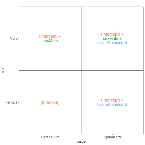
Factorial design with interactions
In the previous model, we assumed that the tissue differences were the same for both male and female mice. To allow for the estimation of sex-specific tissue differences (at the expense of having one additional coefficient to estimate from the data), we can include an interaction term in the model.
R
meta_noninf <- meta %>% filter(time == "Day0")
meta_noninf
OUTPUT
                     title geo_accession     organism     age    sex
GSM2545337 CNS_RNA-seq_11C    GSM2545337 Mus musculus 8 weeks Female
GSM2545338 CNS_RNA-seq_12C    GSM2545338 Mus musculus 8 weeks Female
GSM2545343 CNS_RNA-seq_20C    GSM2545343 Mus musculus 8 weeks   Male
GSM2545348 CNS_RNA-seq_27C    GSM2545348 Mus musculus 8 weeks Female
GSM2545349 CNS_RNA-seq_28C    GSM2545349 Mus musculus 8 weeks   Male
GSM2545353  CNS_RNA-seq_3C    GSM2545353 Mus musculus 8 weeks Female
GSM2545354  CNS_RNA-seq_4C    GSM2545354 Mus musculus 8 weeks   Male
GSM2545356 CNS_RNA-seq_574    GSM2545356 Mus musculus 8 weeks   Male
GSM2545357 CNS_RNA-seq_575    GSM2545357 Mus musculus 8 weeks   Male
GSM2545358 CNS_RNA-seq_583    GSM2545358 Mus musculus 8 weeks Female
GSM2545361 CNS_RNA-seq_590    GSM2545361 Mus musculus 8 weeks   Male
GSM2545364 CNS_RNA-seq_709    GSM2545364 Mus musculus 8 weeks Female
GSM2545365 CNS_RNA-seq_710    GSM2545365 Mus musculus 8 weeks Female
GSM2545366 CNS_RNA-seq_711    GSM2545366 Mus musculus 8 weeks Female
GSM2545367 CNS_RNA-seq_713    GSM2545367 Mus musculus 8 weeks   Male
             infection  strain time     tissue mouse
GSM2545337 NonInfected C57BL/6 Day0 Cerebellum     9
GSM2545338 NonInfected C57BL/6 Day0 Cerebellum    10
GSM2545343 NonInfected C57BL/6 Day0 Cerebellum    11
GSM2545348 NonInfected C57BL/6 Day0 Cerebellum     8
GSM2545349 NonInfected C57BL/6 Day0 Cerebellum     7
GSM2545353 NonInfected C57BL/6 Day0 Cerebellum     4
GSM2545354 NonInfected C57BL/6 Day0 Cerebellum     2
GSM2545356 NonInfected C57BL/6 Day0 Spinalcord     2
GSM2545357 NonInfected C57BL/6 Day0 Spinalcord     3
GSM2545358 NonInfected C57BL/6 Day0 Spinalcord     4
GSM2545361 NonInfected C57BL/6 Day0 Spinalcord     7
GSM2545364 NonInfected C57BL/6 Day0 Spinalcord     8
GSM2545365 NonInfected C57BL/6 Day0 Spinalcord     9
GSM2545366 NonInfected C57BL/6 Day0 Spinalcord    10
GSM2545367 NonInfected C57BL/6 Day0 Spinalcord    11
R
## Define a design including an interaction term
## Note that ~ sex * tissue is equivalent to
## ~ sex + tissue + sex:tissue
vd <- VisualizeDesign(sampleData = meta_noninf,
                      designFormula = ~ sex * tissue)
vd$designmatrix
OUTPUT
           (Intercept) sexMale tissueSpinalcord sexMale:tissueSpinalcord
GSM2545337           1       0                0                        0
GSM2545338           1       0                0                        0
GSM2545343           1       1                0                        0
GSM2545348           1       0                0                        0
GSM2545349           1       1                0                        0
GSM2545353           1       0                0                        0
GSM2545354           1       1                0                        0
GSM2545356           1       1                1                        1
GSM2545357           1       1                1                        1
GSM2545358           1       0                1                        0
GSM2545361           1       1                1                        1
GSM2545364           1       0                1                        0
GSM2545365           1       0                1                        0
GSM2545366           1       0                1                        0
GSM2545367           1       1                1                        1
R
vd$plotlist
OUTPUT
[[1]]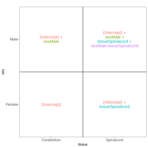
Combining multiple factors into one
Sometimes, for experiments with multiple factors, it is easier to interpret coefficients and set up contrasts of interest if the factors are combined into one. Let’s consider the previous example again, using this approach:
R
meta_noninf <- meta %>% filter(time == "Day0")
meta_noninf$sex_tissue <- paste0(meta_noninf$sex, "_", meta_noninf$tissue)
meta_noninf
OUTPUT
                     title geo_accession     organism     age    sex
GSM2545337 CNS_RNA-seq_11C    GSM2545337 Mus musculus 8 weeks Female
GSM2545338 CNS_RNA-seq_12C    GSM2545338 Mus musculus 8 weeks Female
GSM2545343 CNS_RNA-seq_20C    GSM2545343 Mus musculus 8 weeks   Male
GSM2545348 CNS_RNA-seq_27C    GSM2545348 Mus musculus 8 weeks Female
GSM2545349 CNS_RNA-seq_28C    GSM2545349 Mus musculus 8 weeks   Male
GSM2545353  CNS_RNA-seq_3C    GSM2545353 Mus musculus 8 weeks Female
GSM2545354  CNS_RNA-seq_4C    GSM2545354 Mus musculus 8 weeks   Male
GSM2545356 CNS_RNA-seq_574    GSM2545356 Mus musculus 8 weeks   Male
GSM2545357 CNS_RNA-seq_575    GSM2545357 Mus musculus 8 weeks   Male
GSM2545358 CNS_RNA-seq_583    GSM2545358 Mus musculus 8 weeks Female
GSM2545361 CNS_RNA-seq_590    GSM2545361 Mus musculus 8 weeks   Male
GSM2545364 CNS_RNA-seq_709    GSM2545364 Mus musculus 8 weeks Female
GSM2545365 CNS_RNA-seq_710    GSM2545365 Mus musculus 8 weeks Female
GSM2545366 CNS_RNA-seq_711    GSM2545366 Mus musculus 8 weeks Female
GSM2545367 CNS_RNA-seq_713    GSM2545367 Mus musculus 8 weeks   Male
             infection  strain time     tissue mouse        sex_tissue
GSM2545337 NonInfected C57BL/6 Day0 Cerebellum     9 Female_Cerebellum
GSM2545338 NonInfected C57BL/6 Day0 Cerebellum    10 Female_Cerebellum
GSM2545343 NonInfected C57BL/6 Day0 Cerebellum    11   Male_Cerebellum
GSM2545348 NonInfected C57BL/6 Day0 Cerebellum     8 Female_Cerebellum
GSM2545349 NonInfected C57BL/6 Day0 Cerebellum     7   Male_Cerebellum
GSM2545353 NonInfected C57BL/6 Day0 Cerebellum     4 Female_Cerebellum
GSM2545354 NonInfected C57BL/6 Day0 Cerebellum     2   Male_Cerebellum
GSM2545356 NonInfected C57BL/6 Day0 Spinalcord     2   Male_Spinalcord
GSM2545357 NonInfected C57BL/6 Day0 Spinalcord     3   Male_Spinalcord
GSM2545358 NonInfected C57BL/6 Day0 Spinalcord     4 Female_Spinalcord
GSM2545361 NonInfected C57BL/6 Day0 Spinalcord     7   Male_Spinalcord
GSM2545364 NonInfected C57BL/6 Day0 Spinalcord     8 Female_Spinalcord
GSM2545365 NonInfected C57BL/6 Day0 Spinalcord     9 Female_Spinalcord
GSM2545366 NonInfected C57BL/6 Day0 Spinalcord    10 Female_Spinalcord
GSM2545367 NonInfected C57BL/6 Day0 Spinalcord    11   Male_Spinalcord
R
vd <- VisualizeDesign(sampleData = meta_noninf,
                      designFormula = ~ 0 + sex_tissue)
vd$designmatrix
OUTPUT
           sex_tissueFemale_Cerebellum sex_tissueFemale_Spinalcord
GSM2545337                           1                           0
GSM2545338                           1                           0
GSM2545343                           0                           0
GSM2545348                           1                           0
GSM2545349                           0                           0
GSM2545353                           1                           0
GSM2545354                           0                           0
GSM2545356                           0                           0
GSM2545357                           0                           0
GSM2545358                           0                           1
GSM2545361                           0                           0
GSM2545364                           0                           1
GSM2545365                           0                           1
GSM2545366                           0                           1
GSM2545367                           0                           0
           sex_tissueMale_Cerebellum sex_tissueMale_Spinalcord
GSM2545337                         0                         0
GSM2545338                         0                         0
GSM2545343                         1                         0
GSM2545348                         0                         0
GSM2545349                         1                         0
GSM2545353                         0                         0
GSM2545354                         1                         0
GSM2545356                         0                         1
GSM2545357                         0                         1
GSM2545358                         0                         0
GSM2545361                         0                         1
GSM2545364                         0                         0
GSM2545365                         0                         0
GSM2545366                         0                         0
GSM2545367                         0                         1
R
vd$plotlist
OUTPUT
[[1]]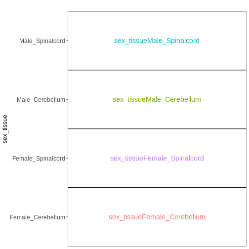
Paired design
In this particular data set the samples are paired - the same mice have contributed both the cerebellum and spinal cord samples. This information was not included in the previous models. However, accounting for it can increase power to detect tissue differences by eliminating variability in baseline expression levels between mice. Here, we define a paired design for the female non-infected mice, aimed at testing for differences between tissues after accounting for baseline differences between mice.
R
meta_fem_day0 <- meta %>% filter(sex == "Female" &
                                     time == "Day0")

# ensure that mouse is treated as a categorical variable
meta_fem_day0$mouse <- factor(meta_fem_day0$mouse)

meta_fem_day0
OUTPUT
                     title geo_accession     organism     age    sex
GSM2545337 CNS_RNA-seq_11C    GSM2545337 Mus musculus 8 weeks Female
GSM2545338 CNS_RNA-seq_12C    GSM2545338 Mus musculus 8 weeks Female
GSM2545348 CNS_RNA-seq_27C    GSM2545348 Mus musculus 8 weeks Female
GSM2545353  CNS_RNA-seq_3C    GSM2545353 Mus musculus 8 weeks Female
GSM2545358 CNS_RNA-seq_583    GSM2545358 Mus musculus 8 weeks Female
GSM2545364 CNS_RNA-seq_709    GSM2545364 Mus musculus 8 weeks Female
GSM2545365 CNS_RNA-seq_710    GSM2545365 Mus musculus 8 weeks Female
GSM2545366 CNS_RNA-seq_711    GSM2545366 Mus musculus 8 weeks Female
             infection  strain time     tissue mouse
GSM2545337 NonInfected C57BL/6 Day0 Cerebellum     9
GSM2545338 NonInfected C57BL/6 Day0 Cerebellum    10
GSM2545348 NonInfected C57BL/6 Day0 Cerebellum     8
GSM2545353 NonInfected C57BL/6 Day0 Cerebellum     4
GSM2545358 NonInfected C57BL/6 Day0 Spinalcord     4
GSM2545364 NonInfected C57BL/6 Day0 Spinalcord     8
GSM2545365 NonInfected C57BL/6 Day0 Spinalcord     9
GSM2545366 NonInfected C57BL/6 Day0 Spinalcord    10
R
vd <- VisualizeDesign(sampleData = meta_fem_day0,
                      designFormula = ~ mouse + tissue)
vd$designmatrix
OUTPUT
           (Intercept) mouse8 mouse9 mouse10 tissueSpinalcord
GSM2545337           1      0      1       0                0
GSM2545338           1      0      0       1                0
GSM2545348           1      1      0       0                0
GSM2545353           1      0      0       0                0
GSM2545358           1      0      0       0                1
GSM2545364           1      1      0       0                1
GSM2545365           1      0      1       0                1
GSM2545366           1      0      0       1                1
R
vd$plotlist
OUTPUT
[[1]]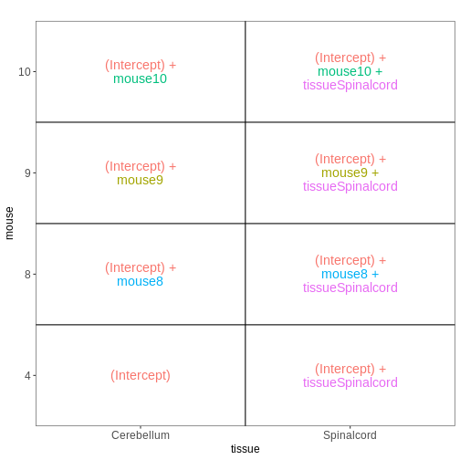
Within- and between-subject comparisons
In some situations, we need to combine the types of models considered above. For example, let’s say that we want to investigate if the tissue differences are different for infected and non-infected female mice. In this case, each mice only contributes to one of the infection groups (each mice is either infected or non-infected), but contributes both a cerebellum and a spinal cord sample. One way to view this type of design is as two paired experiments, one for each infection group (see the edgeR user guide section 3.5). We can then easily compare the two tissues in each infection group, and contrast the tissue differences between the infection groups.
R
meta_fem_day04 <- meta %>%
    filter(sex == "Female" &
               time %in% c("Day0", "Day4")) %>%
    droplevels()
# ensure that mouse is treated as a categorical variable
meta_fem_day04$mouse <- factor(meta_fem_day04$mouse)

meta_fem_day04
OUTPUT
                     title geo_accession     organism     age    sex
GSM2545337 CNS_RNA-seq_11C    GSM2545337 Mus musculus 8 weeks Female
GSM2545338 CNS_RNA-seq_12C    GSM2545338 Mus musculus 8 weeks Female
GSM2545339 CNS_RNA-seq_13C    GSM2545339 Mus musculus 8 weeks Female
GSM2545344 CNS_RNA-seq_21C    GSM2545344 Mus musculus 8 weeks Female
GSM2545348 CNS_RNA-seq_27C    GSM2545348 Mus musculus 8 weeks Female
GSM2545352 CNS_RNA-seq_30C    GSM2545352 Mus musculus 8 weeks Female
GSM2545353  CNS_RNA-seq_3C    GSM2545353 Mus musculus 8 weeks Female
GSM2545358 CNS_RNA-seq_583    GSM2545358 Mus musculus 8 weeks Female
GSM2545362  CNS_RNA-seq_5C    GSM2545362 Mus musculus 8 weeks Female
GSM2545364 CNS_RNA-seq_709    GSM2545364 Mus musculus 8 weeks Female
GSM2545365 CNS_RNA-seq_710    GSM2545365 Mus musculus 8 weeks Female
GSM2545366 CNS_RNA-seq_711    GSM2545366 Mus musculus 8 weeks Female
GSM2545371 CNS_RNA-seq_731    GSM2545371 Mus musculus 8 weeks Female
GSM2545375 CNS_RNA-seq_738    GSM2545375 Mus musculus 8 weeks Female
GSM2545376 CNS_RNA-seq_740    GSM2545376 Mus musculus 8 weeks Female
GSM2545377 CNS_RNA-seq_741    GSM2545377 Mus musculus 8 weeks Female
             infection  strain time     tissue mouse
GSM2545337 NonInfected C57BL/6 Day0 Cerebellum     9
GSM2545338 NonInfected C57BL/6 Day0 Cerebellum    10
GSM2545339  InfluenzaA C57BL/6 Day4 Cerebellum    15
GSM2545344  InfluenzaA C57BL/6 Day4 Cerebellum    22
GSM2545348 NonInfected C57BL/6 Day0 Cerebellum     8
GSM2545352  InfluenzaA C57BL/6 Day4 Cerebellum    21
GSM2545353 NonInfected C57BL/6 Day0 Cerebellum     4
GSM2545358 NonInfected C57BL/6 Day0 Spinalcord     4
GSM2545362  InfluenzaA C57BL/6 Day4 Cerebellum    20
GSM2545364 NonInfected C57BL/6 Day0 Spinalcord     8
GSM2545365 NonInfected C57BL/6 Day0 Spinalcord     9
GSM2545366 NonInfected C57BL/6 Day0 Spinalcord    10
GSM2545371  InfluenzaA C57BL/6 Day4 Spinalcord    15
GSM2545375  InfluenzaA C57BL/6 Day4 Spinalcord    20
GSM2545376  InfluenzaA C57BL/6 Day4 Spinalcord    21
GSM2545377  InfluenzaA C57BL/6 Day4 Spinalcord    22
R
design <- model.matrix(~ mouse, data = meta_fem_day04)
design <- cbind(design,
                Spc.Day0 = meta_fem_day04$tissue == "Spinalcord" &
                    meta_fem_day04$time == "Day0",
                Spc.Day4 = meta_fem_day04$tissue == "Spinalcord" &
                    meta_fem_day04$time == "Day4")
rownames(design) <- rownames(meta_fem_day04)
design
OUTPUT
           (Intercept) mouse8 mouse9 mouse10 mouse15 mouse20 mouse21 mouse22
GSM2545337           1      0      1       0       0       0       0       0
GSM2545338           1      0      0       1       0       0       0       0
GSM2545339           1      0      0       0       1       0       0       0
GSM2545344           1      0      0       0       0       0       0       1
GSM2545348           1      1      0       0       0       0       0       0
GSM2545352           1      0      0       0       0       0       1       0
GSM2545353           1      0      0       0       0       0       0       0
GSM2545358           1      0      0       0       0       0       0       0
GSM2545362           1      0      0       0       0       1       0       0
GSM2545364           1      1      0       0       0       0       0       0
GSM2545365           1      0      1       0       0       0       0       0
GSM2545366           1      0      0       1       0       0       0       0
GSM2545371           1      0      0       0       1       0       0       0
GSM2545375           1      0      0       0       0       1       0       0
GSM2545376           1      0      0       0       0       0       1       0
GSM2545377           1      0      0       0       0       0       0       1
           Spc.Day0 Spc.Day4
GSM2545337        0        0
GSM2545338        0        0
GSM2545339        0        0
GSM2545344        0        0
GSM2545348        0        0
GSM2545352        0        0
GSM2545353        0        0
GSM2545358        1        0
GSM2545362        0        0
GSM2545364        1        0
GSM2545365        1        0
GSM2545366        1        0
GSM2545371        0        1
GSM2545375        0        1
GSM2545376        0        1
GSM2545377        0        1
R
vd <- VisualizeDesign(sampleData = meta_fem_day04 %>%
                          select(time, tissue, mouse),
                      designFormula = NULL,
                      designMatrix = design, flipCoordFitted = FALSE)
vd$designmatrix
OUTPUT
           (Intercept) mouse8 mouse9 mouse10 mouse15 mouse20 mouse21 mouse22
GSM2545337           1      0      1       0       0       0       0       0
GSM2545338           1      0      0       1       0       0       0       0
GSM2545339           1      0      0       0       1       0       0       0
GSM2545344           1      0      0       0       0       0       0       1
GSM2545348           1      1      0       0       0       0       0       0
GSM2545352           1      0      0       0       0       0       1       0
GSM2545353           1      0      0       0       0       0       0       0
GSM2545358           1      0      0       0       0       0       0       0
GSM2545362           1      0      0       0       0       1       0       0
GSM2545364           1      1      0       0       0       0       0       0
GSM2545365           1      0      1       0       0       0       0       0
GSM2545366           1      0      0       1       0       0       0       0
GSM2545371           1      0      0       0       1       0       0       0
GSM2545375           1      0      0       0       0       1       0       0
GSM2545376           1      0      0       0       0       0       1       0
GSM2545377           1      0      0       0       0       0       0       1
           Spc.Day0 Spc.Day4
GSM2545337        0        0
GSM2545338        0        0
GSM2545339        0        0
GSM2545344        0        0
GSM2545348        0        0
GSM2545352        0        0
GSM2545353        0        0
GSM2545358        1        0
GSM2545362        0        0
GSM2545364        1        0
GSM2545365        1        0
GSM2545366        1        0
GSM2545371        0        1
GSM2545375        0        1
GSM2545376        0        1
GSM2545377        0        1
R
vd$plotlist
OUTPUT
$`time = Day0`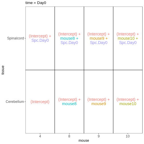
OUTPUT
$`time = Day4`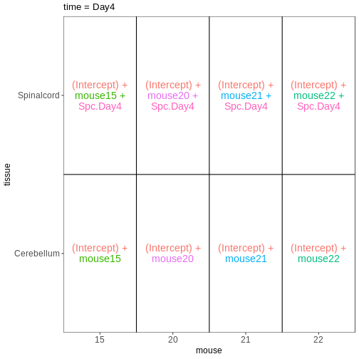
How does this relate to the DESeq2 analysis we did in the previous episode?
Now that we have learnt more about interpreting design matrices, let’s look back to the differential expression analysis we performed in the previous episode. We will repeat the main lines of code here.
R
se <- readRDS("data/GSE96870_se.rds")
se <- se[rowSums(assay(se, "counts")) > 5, ]
dds <- DESeq2::DESeqDataSet(se, design = ~ sex + time)
dds <- DESeq(dds)
OUTPUT
estimating size factorsOUTPUT
estimating dispersionsOUTPUT
gene-wise dispersion estimatesOUTPUT
mean-dispersion relationshipOUTPUT
final dispersion estimatesOUTPUT
fitting model and testingDESeq2 stores the design matrix in the object:
R
attr(dds, "modelMatrix")
OUTPUT
               Intercept sex_Male_vs_Female time_Day4_vs_Day0 time_Day8_vs_Day0
Female_Day0_9          1                  0                 0                 0
Female_Day0_10         1                  0                 0                 0
Female_Day0_8          1                  0                 0                 0
Female_Day0_4          1                  0                 0                 0
Male_Day0_11           1                  1                 0                 0
Male_Day0_7            1                  1                 0                 0
Male_Day0_2            1                  1                 0                 0
Female_Day4_15         1                  0                 1                 0
Female_Day4_22         1                  0                 1                 0
Female_Day4_21         1                  0                 1                 0
Female_Day4_20         1                  0                 1                 0
Male_Day4_18           1                  1                 1                 0
Male_Day4_13           1                  1                 1                 0
Male_Day4_1            1                  1                 1                 0
Male_Day4_12           1                  1                 1                 0
Female_Day8_14         1                  0                 0                 1
Female_Day8_5          1                  0                 0                 1
Female_Day8_16         1                  0                 0                 1
Female_Day8_19         1                  0                 0                 1
Male_Day8_6            1                  1                 0                 1
Male_Day8_23           1                  1                 0                 1
Male_Day8_24           1                  1                 0                 1
attr(,"assign")
[1] 0 1 2 2
attr(,"contrasts")
attr(,"contrasts")$sex
[1] "contr.treatment"

attr(,"contrasts")$time
[1] "contr.treatment"
The column names can be obtained via the resultsNames
function:
R
resultsNames(dds)
OUTPUT
[1] "Intercept"          "sex_Male_vs_Female" "time_Day4_vs_Day0"
[4] "time_Day8_vs_Day0"
Let’s visualize this design:
R
vd <- VisualizeDesign(sampleData = colData(dds)[, c("sex", "time")],
                      designMatrix = attr(dds, "modelMatrix"),
                      flipCoordFitted = TRUE)
vd$plotlist
OUTPUT
[[1]]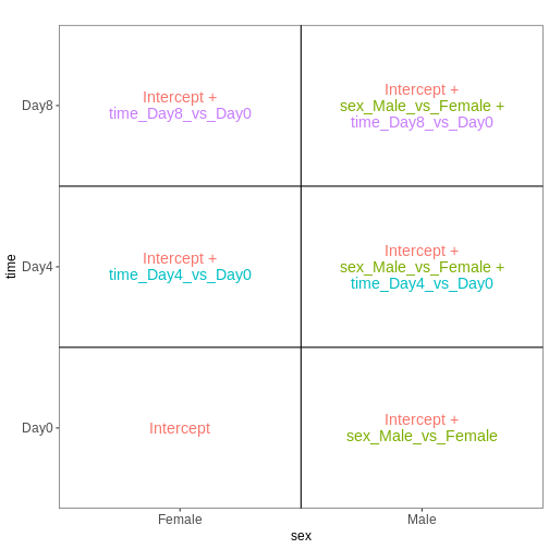
In the previous episode, we performed a test comparing Day8 samples to Day0 samples:
R
resTime <- results(dds, contrast = c("time", "Day8", "Day0"))
From the figure above, we see that this comparison is represented by
the time_Day8_vs_Day0 coefficient, which corresponds to the
fourth column in the design matrix. Thus, an alternative way of
specifying the contrast for the test would be:
R
resTimeNum <- results(dds, contrast = c(0, 0, 0, 1))
Let’s check if the results are comparable:
R
summary(resTime)
OUTPUT
out of 27430 with nonzero total read count
adjusted p-value < 0.1
LFC > 0 (up)       : 4472, 16%
LFC < 0 (down)     : 4282, 16%
outliers [1]       : 10, 0.036%
low counts [2]     : 3723, 14%
(mean count < 1)
[1] see 'cooksCutoff' argument of ?results
[2] see 'independentFiltering' argument of ?results
R
summary(resTimeNum)
OUTPUT
out of 27430 with nonzero total read count
adjusted p-value < 0.1
LFC > 0 (up)       : 4472, 16%
LFC < 0 (down)     : 4282, 16%
outliers [1]       : 10, 0.036%
low counts [2]     : 3723, 14%
(mean count < 1)
[1] see 'cooksCutoff' argument of ?results
[2] see 'independentFiltering' argument of ?results
R
## logFC
plot(resTime$log2FoldChange, resTimeNum$log2FoldChange)
abline(0, 1)
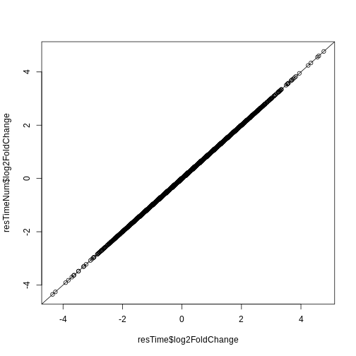
R
## -log10(p-value)
plot(-log10(resTime$pvalue), -log10(resTimeNum$pvalue))
abline(0, 1)
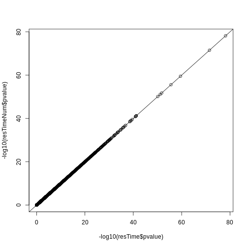
Redo DESeq2 analysis with interaction
Next, let’s look at a different setup. We still consider the sex and time predictors, but now we allow an interaction between them. In other words, we allow the time effect to be different for males and females.
R
se <- readRDS("data/GSE96870_se.rds")
se <- se[rowSums(assay(se, "counts")) > 5, ]
dds <- DESeq2::DESeqDataSet(se, design = ~ sex * time)
dds <- DESeq(dds)
OUTPUT
estimating size factorsOUTPUT
estimating dispersionsOUTPUT
gene-wise dispersion estimatesOUTPUT
mean-dispersion relationshipOUTPUT
final dispersion estimatesOUTPUT
fitting model and testingR
attr(dds, "modelMatrix")
OUTPUT
               Intercept sex_Male_vs_Female time_Day4_vs_Day0 time_Day8_vs_Day0
Female_Day0_9          1                  0                 0                 0
Female_Day0_10         1                  0                 0                 0
Female_Day0_8          1                  0                 0                 0
Female_Day0_4          1                  0                 0                 0
Male_Day0_11           1                  1                 0                 0
Male_Day0_7            1                  1                 0                 0
Male_Day0_2            1                  1                 0                 0
Female_Day4_15         1                  0                 1                 0
Female_Day4_22         1                  0                 1                 0
Female_Day4_21         1                  0                 1                 0
Female_Day4_20         1                  0                 1                 0
Male_Day4_18           1                  1                 1                 0
Male_Day4_13           1                  1                 1                 0
Male_Day4_1            1                  1                 1                 0
Male_Day4_12           1                  1                 1                 0
Female_Day8_14         1                  0                 0                 1
Female_Day8_5          1                  0                 0                 1
Female_Day8_16         1                  0                 0                 1
Female_Day8_19         1                  0                 0                 1
Male_Day8_6            1                  1                 0                 1
Male_Day8_23           1                  1                 0                 1
Male_Day8_24           1                  1                 0                 1
               sexMale.timeDay4 sexMale.timeDay8
Female_Day0_9                 0                0
Female_Day0_10                0                0
Female_Day0_8                 0                0
Female_Day0_4                 0                0
Male_Day0_11                  0                0
Male_Day0_7                   0                0
Male_Day0_2                   0                0
Female_Day4_15                0                0
Female_Day4_22                0                0
Female_Day4_21                0                0
Female_Day4_20                0                0
Male_Day4_18                  1                0
Male_Day4_13                  1                0
Male_Day4_1                   1                0
Male_Day4_12                  1                0
Female_Day8_14                0                0
Female_Day8_5                 0                0
Female_Day8_16                0                0
Female_Day8_19                0                0
Male_Day8_6                   0                1
Male_Day8_23                  0                1
Male_Day8_24                  0                1
attr(,"assign")
[1] 0 1 2 2 3 3
attr(,"contrasts")
attr(,"contrasts")$sex
[1] "contr.treatment"

attr(,"contrasts")$time
[1] "contr.treatment"
Let’s visualize this design:
R
vd <- VisualizeDesign(sampleData = colData(dds)[, c("sex", "time")],
                      designMatrix = attr(dds, "modelMatrix"),
                      flipCoordFitted = TRUE)
vd$plotlist
OUTPUT
[[1]]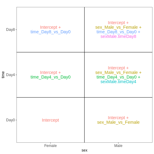
Note that now, the time_Day8_vs_Day0 coefficient
represents the difference between Day8 and Day0 for the Female
samples. To get the corresponding difference for the male
samples, we need to also add the interaction effect
(sexMale.timeDay8).
R
## Day8 vs Day0, female
resTimeFemale <- results(dds, contrast = c("time", "Day8", "Day0"))

## Interaction effect (difference in Day8-Day0 effect between Male and Female)
resTimeInt <- results(dds, name = "sexMale.timeDay8")
Let’s try to fit this model with the second approach mentioned above, namely to create a single factor.
R
se <- readRDS("data/GSE96870_se.rds")
se <- se[rowSums(assay(se, "counts")) > 5, ]
se$sex_time <- paste0(se$sex, "_", se$time)
dds <- DESeq2::DESeqDataSet(se, design = ~ 0 + sex_time)
dds <- DESeq(dds)
OUTPUT
estimating size factorsOUTPUT
estimating dispersionsOUTPUT
gene-wise dispersion estimatesOUTPUT
mean-dispersion relationshipOUTPUT
final dispersion estimatesOUTPUT
fitting model and testingR
attr(dds, "modelMatrix")
OUTPUT
               sex_timeFemale_Day0 sex_timeFemale_Day4 sex_timeFemale_Day8
Female_Day0_9                    1                   0                   0
Female_Day0_10                   1                   0                   0
Female_Day0_8                    1                   0                   0
Female_Day0_4                    1                   0                   0
Male_Day0_11                     0                   0                   0
Male_Day0_7                      0                   0                   0
Male_Day0_2                      0                   0                   0
Female_Day4_15                   0                   1                   0
Female_Day4_22                   0                   1                   0
Female_Day4_21                   0                   1                   0
Female_Day4_20                   0                   1                   0
Male_Day4_18                     0                   0                   0
Male_Day4_13                     0                   0                   0
Male_Day4_1                      0                   0                   0
Male_Day4_12                     0                   0                   0
Female_Day8_14                   0                   0                   1
Female_Day8_5                    0                   0                   1
Female_Day8_16                   0                   0                   1
Female_Day8_19                   0                   0                   1
Male_Day8_6                      0                   0                   0
Male_Day8_23                     0                   0                   0
Male_Day8_24                     0                   0                   0
               sex_timeMale_Day0 sex_timeMale_Day4 sex_timeMale_Day8
Female_Day0_9                  0                 0                 0
Female_Day0_10                 0                 0                 0
Female_Day0_8                  0                 0                 0
Female_Day0_4                  0                 0                 0
Male_Day0_11                   1                 0                 0
Male_Day0_7                    1                 0                 0
Male_Day0_2                    1                 0                 0
Female_Day4_15                 0                 0                 0
Female_Day4_22                 0                 0                 0
Female_Day4_21                 0                 0                 0
Female_Day4_20                 0                 0                 0
Male_Day4_18                   0                 1                 0
Male_Day4_13                   0                 1                 0
Male_Day4_1                    0                 1                 0
Male_Day4_12                   0                 1                 0
Female_Day8_14                 0                 0                 0
Female_Day8_5                  0                 0                 0
Female_Day8_16                 0                 0                 0
Female_Day8_19                 0                 0                 0
Male_Day8_6                    0                 0                 1
Male_Day8_23                   0                 0                 1
Male_Day8_24                   0                 0                 1
attr(,"assign")
[1] 1 1 1 1 1 1
attr(,"contrasts")
attr(,"contrasts")$sex_time
[1] "contr.treatment"
We again visualize this design:
R
vd <- VisualizeDesign(sampleData = colData(dds)[, c("sex", "time")],
                      designMatrix = attr(dds, "modelMatrix"),
                      flipCoordFitted = TRUE)
vd$plotlist
OUTPUT
[[1]]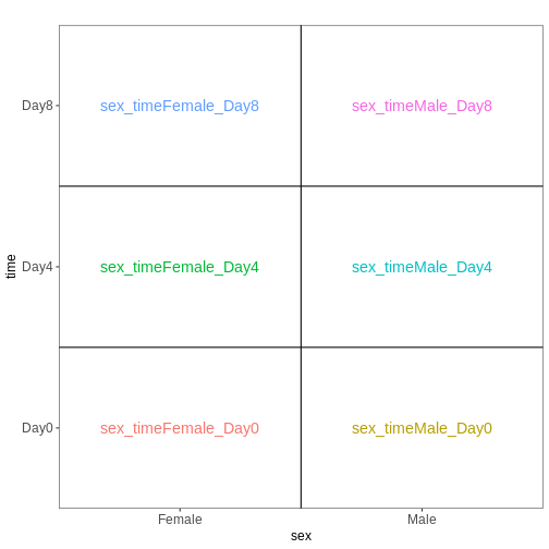
We then set up the same contrasts as above
R
## Day8 vs Day0, female
resTimeFemaleSingle <- results(dds, contrast = c("sex_time", "Female_Day8", "Female_Day0"))

## Interaction effect (difference in Day8-Day0 effect between Male and Female)
resultsNames(dds)
OUTPUT
[1] "sex_timeFemale_Day0" "sex_timeFemale_Day4" "sex_timeFemale_Day8"
[4] "sex_timeMale_Day0"   "sex_timeMale_Day4"   "sex_timeMale_Day8"
R
resTimeIntSingle <- results(dds, contrast = c(1, 0, -1, -1, 0, 1))
Check that these results agree with the ones obtained by fitting the model with the two factors and the interaction term.
R
summary(resTimeFemale)
OUTPUT
out of 27430 with nonzero total read count
adjusted p-value < 0.1
LFC > 0 (up)       : 2969, 11%
LFC < 0 (down)     : 3218, 12%
outliers [1]       : 6, 0.022%
low counts [2]     : 6382, 23%
(mean count < 3)
[1] see 'cooksCutoff' argument of ?results
[2] see 'independentFiltering' argument of ?results
R
summary(resTimeFemaleSingle)
OUTPUT
out of 27430 with nonzero total read count
adjusted p-value < 0.1
LFC > 0 (up)       : 2969, 11%
LFC < 0 (down)     : 3218, 12%
outliers [1]       : 6, 0.022%
low counts [2]     : 6382, 23%
(mean count < 3)
[1] see 'cooksCutoff' argument of ?results
[2] see 'independentFiltering' argument of ?results
R
plot(-log10(resTimeFemale$pvalue), -log10(resTimeFemaleSingle$pvalue))
abline(0, 1)
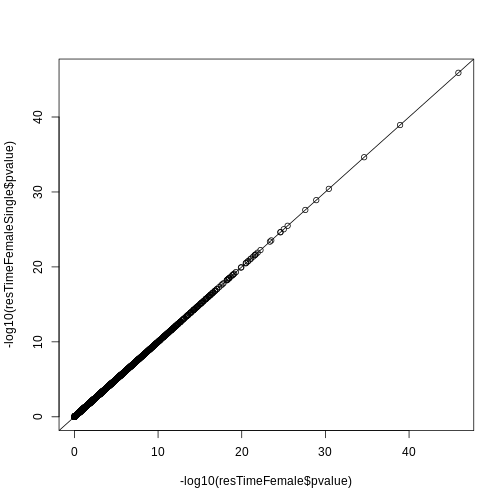
R
summary(resTimeInt)
OUTPUT
out of 27430 with nonzero total read count
adjusted p-value < 0.1
LFC > 0 (up)       : 0, 0%
LFC < 0 (down)     : 0, 0%
outliers [1]       : 6, 0.022%
low counts [2]     : 0, 0%
(mean count < 0)
[1] see 'cooksCutoff' argument of ?results
[2] see 'independentFiltering' argument of ?results
R
summary(resTimeIntSingle)
OUTPUT
out of 27430 with nonzero total read count
adjusted p-value < 0.1
LFC > 0 (up)       : 0, 0%
LFC < 0 (down)     : 0, 0%
outliers [1]       : 6, 0.022%
low counts [2]     : 0, 0%
(mean count < 0)
[1] see 'cooksCutoff' argument of ?results
[2] see 'independentFiltering' argument of ?results
R
plot(-log10(resTimeInt$pvalue), -log10(resTimeIntSingle$pvalue))
abline(0, 1)
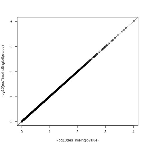
- The formula framework in R allows creation of design matrices, which details the variables expected to be associated with systematic differences in gene expression levels.
- Comparisons of interest can be defined using contrasts, which are linear combinations of the model coefficients.
Content from Gene set enrichment analysis
Last updated on 2025-11-11 | Edit this page
Estimated time 105 minutes
Overview
Questions
- What is the aim of performing gene set enrichment analysis?
- What is the method of over-representation analysis?
- What are the commonly-used gene set databases?
Objectives
- Learn the method of gene set enrichment analysis.
- Learn how to obtain gene sets from various resources in R.
- Learn how to perform gene set enrichment analysis and how to visualize enrichment results.
After we have obtained a list of differentially expressed (DE) genes, the next question naturally to ask is what biological functions these DE genes may affect. Gene set enrichment analysis (GSEA) evaluates the associations of a list of DE genes to a collection of pre-defined gene sets, where each gene set has a specific biological meaning. Once DE genes are significantly enriched in a gene set, the conclusion is made that the corresponding biological meaning (e.g. a biological process or a pathway) is significantly affected.
The definition of a gene set is very flexible and the construction of gene sets is straightforward. In most cases, gene sets are from public databases where huge efforts from scientific curators have already been made to carefully categorize genes into gene sets with clear biological meanings. Nevertheless, gene sets can also be self-defined from individual studies, such as a set of genes in a network module from a co-expression network analysis, or a set of genes that are up-regulated in a certain disease.
There are a huge amount of methods available for GSEA analysis. In this episode, we will learn the simplest but the mostly used one: the over-representation analysis (ORA). ORA is directly applied to the list of DE genes and it evaluates the association of the DE genes and the gene set by the numbers of genes in different categories.
Please note, ORA is a universal method that it can not only be applied to the DE gene list, but also any type of gene list of interest to look for their statistically associated biological meanings.
In this episode, we will start with a tiny example to illustrate the statistical method of ORA. Next we will go through several commonly-used gene set databases and how to access them in R. Then, we will learn how to perform ORA analysis with the Bioconductor package clusterProfiler. And in the end, we will learn several visualization methods on the GSEA results.
Following is a list of packages that will be used in this episode:
R
library(SummarizedExperiment)
library(DESeq2)
library(gplots)
library(microbenchmark)
library(org.Hs.eg.db)
library(org.Mm.eg.db)
library(msigdb)
library(clusterProfiler)
library(enrichplot)
library(ggplot2)
library(simplifyEnrichment)
The statistical method
To demonstrate the ORA analysis, we use a list of DE genes from a
comparison between genders. The following code performs
DESeq2 analysis which you should have already learnt in
the previous episode. In the end, we have a list of DE genes filtered by
FDR < 0.05, and save it in the object sexDEgenes.
The file data/GSE96870_se.rds contains a
RangedSummarizedExperiment that contains RNA-Seq counts
that were downloaded in Episode 2 and
constructed in Episode 3 (minimal
codes for downloading and constructing in the script download_data.R.
In the following code, there are also comments that explain every step
of the analysis.
R
library(SummarizedExperiment)
library(DESeq2)

# read the example dataset which is a `RangedSummarizedExperiment` object
se <- readRDS("data/GSE96870_se.rds")

# only restrict to mRNA (protein-coding genes)
se <- se[rowData(se)$gbkey == "mRNA"]

# construct a `DESeqDataSet` object where we also specify the experimental design
dds <- DESeqDataSet(se, design = ~ sex + time)
# perform DESeq2 analysis
dds <- DESeq(dds)
# obtain DESeq2 results, here we only want Male vs Female in the "sex" variable
resSex <- results(dds, contrast = c("sex", "Male", "Female"))
# extract DE genes with padj < 0.05
sexDE <- as.data.frame(subset(resSex, padj < 0.05))
# the list of DE genes
sexDEgenes <- rownames(sexDE)
Let’s check the number of DE genes and how they look like. It seems the number of DE genes is very small, but it is OK for this example.
R
length(sexDEgenes)
OUTPUT
[1] 54R
head(sexDEgenes)
OUTPUT
[1] "Lgr6" "Myoc" "Fibcd1" "Kcna4" "Ctxn2" "S100a9"Next we construct a gene set which contains genes on sex chromosomes
(let’s call it the “XY gene set”). Recall the
RangedSummarizedExperiment object also includes genomic
locations of genes, thus we can simply obtain sex genes by filtering the
chromosome names.
In the following code, geneGR is a GRanges
object on which seqnames() is applied to extract chromosome
names. seqnames() returns a special data format and we need
to explicitly convert it to a normal vector by
as.vector().
R
geneGR <- rowRanges(se)
totalGenes <- rownames(se)
XYGeneSet <- totalGenes[as.vector(seqnames(geneGR)) %in% c("X", "Y")]
head(XYGeneSet)
OUTPUT
[1] "Gm21950" "Gm14346" "Gm14345" "Gm14351" "Spin2-ps1" "Gm3701" R
length(XYGeneSet)
OUTPUT
[1] 1134The format of a single gene set is very straightforward, which is simply a vector. The ORA analysis is applied on the DE gene vector and gene set vector.
Before we move on, one thing worth to mention is that ORA deals with
two gene vectors. To correctly map between them, gene ID types must be
consistent in the two vectors. In this tiny example, since both DE genes
and the XY gene set are from the same object se,
they are ensured to be in the same gene ID types (the gene symbol). But
in general, DE genes and gene sets are from two different sources
(e.g. DE genes are from researcher’s experiment and gene sets are from
public databases), it is very possible that gene IDs are not consistent
in the two. Later in this episode, we will learn how to perform gene ID
conversion in the ORA analysis.
Since the DE genes and the gene set can be mathematically thought of as two sets, a natural way is to first visualize them with a Venn diagram.
R
library(gplots)
plot(venn(list("sexDEgenes"  = sexDEgenes,
               "XY gene set" = XYGeneSet)))
title(paste0("|universe| = ", length(totalGenes)))
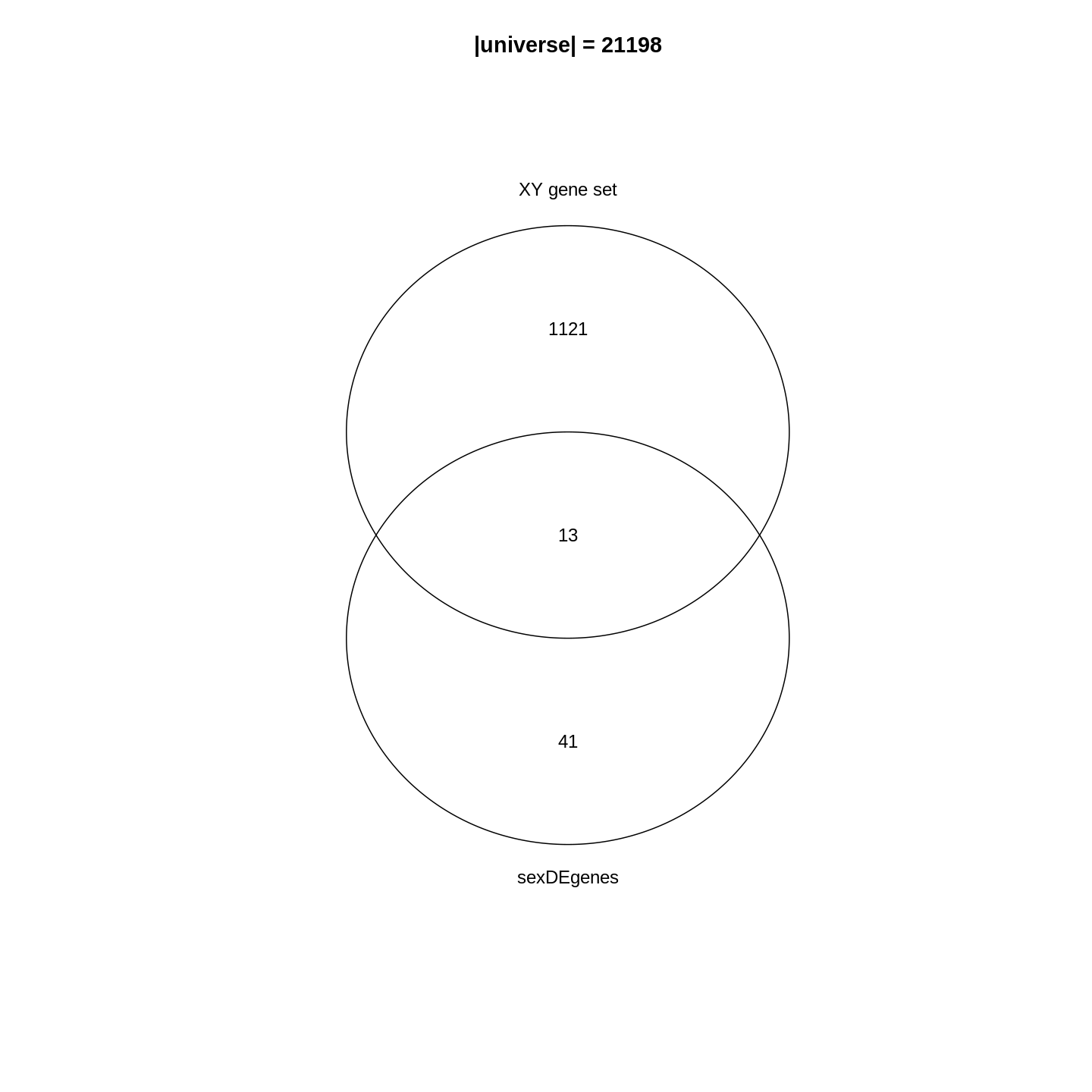
In the Venn diagram, we can observe that around 1.1% (13/1134) of genes in the XY gene set are DE. Compared to the global fraction of DE genes (54/21198 = 0.25%), it seems there is a strong relations between DE genes and the gene set. We can also compare the fraction of DE genes that belong to the gene set (13/54 = 24.1%) and the global fraction of XY gene set in the genome (1134/21198 = 5.3%). On the other hand, it is quite expected because the two events are actually biologically relevant where one is from a comparison between genders and the other is the set of gender-related genes.
Then, how to statistically measure the enrichment or over-representation? Let’s go to the next section.
Fisher’s exact test
To statistically measure the enrichment, the relationship of DE genes and the gene set is normally formatted into the following 2x2 contingency table, where in the table are the numbers of genes in different categories. \(n_{+1}\) is the size of the XY gene set (i.e. the number of member genes), \(n_{1+}\) is the number of DE genes, \(n\) is the number of total genes.
| In the gene set | Not in the gene set | Total | |
|---|---|---|---|
| DE | \(n_{11}\) | \(n_{12}\) | \(n_{1+}\) |
| Not DE | \(n_{21}\) | \(n_{22}\) | \(n_{2+}\) |
| Total | \(n_{+1}\) | \(n_{+2}\) | \(n\) |
These numbers can be obtained as in the following code1. Note we replace
+ with 0 in the R variable names.
R
n    <- nrow(se)
n_01 <- length(XYGeneSet)
n_10 <- length(sexDEgenes)
n_11 <- length(intersect(sexDEgenes, XYGeneSet))
Other values can be obtained by:
R
n_12 <- n_10 - n_11
n_21 <- n_01 - n_11
n_20 <- n    - n_10
n_02 <- n    - n_01
n_22 <- n_02 - n_12
All the values are:
R
matrix(c(n_11, n_12, n_10, n_21, n_22, n_20, n_01, n_02, n),
    nrow = 3, byrow = TRUE)
OUTPUT
     [,1]  [,2]  [,3]
[1,]   13    41    54
[2,] 1121 20023 21144
[3,] 1134 20064 21198
And we fill these numbers into the 2x2 contingency table:
| In the gene set | Not in the gene set | Total | |
|---|---|---|---|
| DE | 13 | 41 | 54 |
| Not DE | 1121 | 20023 | 21144 |
| Total | 1134 | 20064 | 21198 |
Fisher’s exact test can be used to test the associations of the two
marginal attributes, i.e. is there a dependency of a gene to be a DE
gene and to be in the XY gene set? In R, we can use the
function fisher.test() to perform the test. The input is
the top-left 2x2 sub-matrix. We specify
alternative = "greater" in the function because we are only
interested in over-representation.
R
fisher.test(matrix(c(n_11, n_12, n_21, n_22), nrow = 2, byrow = TRUE),
    alternative = "greater")
OUTPUT
	Fisher's Exact Test for Count Data

data:  matrix(c(n_11, n_12, n_21, n_22), nrow = 2, byrow = TRUE)
p-value = 3.906e-06
alternative hypothesis: true odds ratio is greater than 1
95 percent confidence interval:
 3.110607      Inf
sample estimates:
odds ratio
  5.662486
In the output, we can see the p-value is very small
(3.906e-06), then we can conclude DE genes have a very
strong enrichment in the XY gene set.
Results of the Fisher’s Exact test can be saved into an object
t, which is a simple list, and the p-value can be
obtained by t$p.value.
R
t <- fisher.test(matrix(c(n_11, n_12, n_21, n_22), nrow = 2, byrow = TRUE),
    alternative = "greater")
t$p.value
OUTPUT
[1] 3.9059e-06Odds ratio from the Fisher’s exact test is defined as follows:
\[ \mathrm{Odds\_ratio} = \frac{n_{11}/n_{21}}{n_{12}/n_{22}} = \frac{n_{11}/n_{12}}{n_{21}/n_{22}} = \frac{n_{11} * n_{22}}{n_{12} * n_{21}} \]
If there is no association between DE genes and the gene set, odds ratio is expected to be 1. And it is larger than 1 if there is an over-representation of DE genes on the gene set.
Further reading
The 2x2 contingency table can be transposed and it does not affect the Fisher’s exact test. E.g. let’s put whether genes are in the gene sets on rows, and put whether genes are DE on columns.
| DE | Not DE | Total | |
|---|---|---|---|
| In the gene set | 13 | 1121 | 1134 |
| Not in the gene set | 41 | 20023 | 20064 |
| Total | 54 | 21144 | 21198 |
And the corresponding fisher.test() is:
R
fisher.test(matrix(c(13, 1121, 41, 20023), nrow = 2, byrow = TRUE),
    alternative = "greater")
OUTPUT
	Fisher's Exact Test for Count Data

data:  matrix(c(13, 1121, 41, 20023), nrow = 2, byrow = TRUE)
p-value = 3.906e-06
alternative hypothesis: true odds ratio is greater than 1
95 percent confidence interval:
 3.110607      Inf
sample estimates:
odds ratio
  5.662486
The hypergeometric distribution
We can look at the problem from another aspect. This time we treat all genes as balls in a big box where all the genes have the same probability to be picked up. Some genes are marked as DE genes (in red in the figure) and other genes are marked as non-DE genes (in blue). We grab \(n_{+1}\) genes (the size of the gene set) from the box and we want to ask what is the probability of having \(n_{11}\) DE genes in our hand?
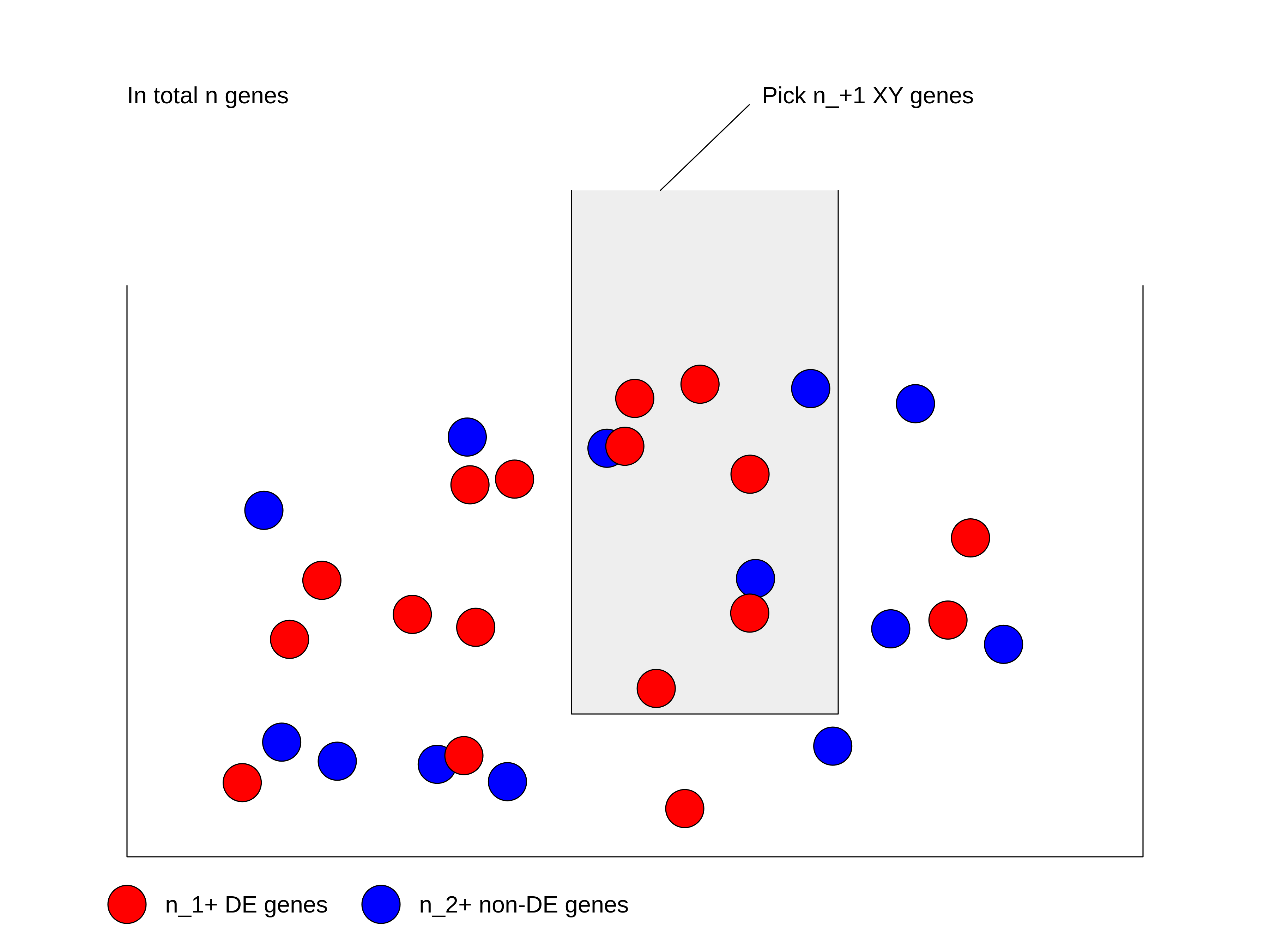
We first calculate the total number of ways of picking \(n_{+1}\) genes from total \(n\) genes, without distinguishing whether they are DE or not: \(\binom{n}{n_{+1}}\).
Next, in the \(n_{+1}\) genes that have been picked, there are \(n_{11}\) DE genes which can only be from the total \(n_{1+}\) DE genes. Then the number of ways of picking \(n_{11}\) DE genes from \(n_{1+}\) total DE genes is \(\binom{n_{1+}}{n_{11}}\).
Similarly, there are still \(n_{21}\) non-DE genes in our hand, which can only be from the total \(n_{2+}\) non-DE genes. Then the number of ways of picking \(n_{21}\) non-DE genes from \(n_{2+}\) total non-DE genes: \(\binom{n_{2+}}{n_{21}}\).
Since picking DE genes and picking non-DE genes are independent, the number of ways of picking \(n_{+1}\) genes which contain \(n_{11}\) DE genes and \(n_{21}\) non-DE genes is their multiplication: \(\binom{n_{1+}}{n_{11}} \binom{n_{2+}}{n_{21}}\).
And the probability \(P\) is:
\[P = \frac{\binom{n_{1+}}{n_{11}} \binom{n_{2+}}{n_{21}}}{\binom{n}{n_{+1}}} = \frac{\binom{n_{1+}}{n_{11}} \binom{n - n_{1+}}{n_{+1} -n_{11}}}{\binom{n}{n_{+1}}} \]
where in the denominator is the number of ways of picking \(n_{+1}\) genes without distinguishing whether they are DE or not.
If \(n\) (number of total genes), \(n_{1+}\) (number of DE genes) and \(n_{+1}\) (size of gene set) are all fixed values, the number of DE genes that are picked can be denoted as a random variable \(X\). Then \(X\) follows the hypergeometric distribution with parameters \(n\), \(n_{1+}\) and \(n_{+1}\), written as:
\[ X \sim \mathrm{Hyper}(n, n_{1+}, n_{+1})\]
The p-value of the enrichment is calculated as the probability of having an observation equal to or larger than \(n_{11}\) under the assumption of independence:
\[ \mathrm{Pr}( X \geqslant n_{11} ) = \sum_{x \in \{ {n_{11}, n_{11}+1, ..., \min\{n_{1+}, n_{+1}\} \}}} \mathrm{Pr}(X = x) \]
In R, the function phyper() calculates p-values
from the hypergeometric distribution. There are four arguments:
R
phyper(q, m, n, k)
which are:
-
q: the observation, -
m: number of DE genes, -
n: number of non-DE genes, -
k: size of the gene set.
phyper() calculates \(\mathrm{Pr}(X \leqslant q)\). To calculate
\(\mathrm{Pr}(X \geqslant q)\), we need
to transform it a little bit:
\[ \mathrm{Pr}(X \geqslant q) = 1 - \mathrm{Pr}(X < q) = 1 - \mathrm{Pr}(X \leqslant q-1)\]
Then, the correct use of phyper() is:
R
1 - phyper(q - 1, m, n, k)
Let’s plugin our variables:
R
1 - phyper(n_11 - 1, n_10, n_20, n_01)
OUTPUT
[1] 3.9059e-06Optionally, lower.tail argument can be specified which
directly calculates p-values from the upper tail of the
distribution.
R
phyper(n_11 - 1, n_10, n_20, n_01, lower.tail = FALSE)
OUTPUT
[1] 3.9059e-06If we switch n_01 and n_10, the
p-values are identical:
R
1 - phyper(n_11 - 1, n_01, n_02, n_10)
OUTPUT
[1] 3.9059e-06fisher.test() and phyper() give the same
p-value. Actually the two methods are identical because in
Fisher’s exact test, hypergeometric distribution is the exact
distribution of its statistic.
Let’s test the runtime of the two functions:
R
library(microbenchmark)
microbenchmark(
    fisher = fisher.test(matrix(c(n_11, n_12, n_21, n_22), nrow = 2, byrow = TRUE),
        alternative = "greater"),
    hyper = 1 - phyper(n_11 - 1, n_10, n_20, n_01)
)
OUTPUT
Unit: microseconds
   expr     min       lq      mean   median      uq     max neval
 fisher 252.671 260.1000 271.52655 264.2125 277.633 503.499   100
  hyper   1.593   1.6835   2.57897   1.9135   3.091  20.548   100
It is very astonishing that phyper() is hundreds of
times faster than fisher.test(). Main reason is in
fisher.test(), there are many additional calculations
besides calculating the p-value. So if you want to implement
ORA analysis by yourself, always consider to use phyper()2.
Further reading
Current tools also use Binomial distribution or chi-square test for ORA analysis. These two are just approximations. Please refer to Rivals et al., Enrichment or depletion of a GO category within a class of genes: which test? Bioinformatics 2007 which gives an overview of statistical methods used in ORA analysis.
Gene set resources
We have learnt the basic methods of ORA analysis. Now we go to the second component of the analysis: the gene sets.
Gene sets represent prior knowledge of what is the general shared biological attribute of genes in the gene set. For example, in a “cell cycle” gene set, all the genes are involved in the cell cycle process. Thus, if DE genes are significantly enriched in the “cell cycle” gene set, which means there are significantly more cell cycle genes differentially expressed than expected, we can conclude that the normal function of cell cycle process may be affected.
As we have mentioned, genes in the gene set share the same “biological attribute” where “the attribute” will be used for making conclusions. The definition of “biological attribute” is very flexible. It can be a biological process such as “cell cycle”. It can also be from a wide range of other definitions, to name a few:
- Locations in the cell, e.g. cell membrane or cell nucleus.
- Positions on chromosomes, e.g. sex chromosomes or the cytogenetic band p13 on chromome 10.
- Target genes of a transcription factor or a microRNA, e.g. all genes that are transcriptionally regulationed by NF-κB.
- Signature genes in a certain tumor type, i.e. genes that are uniquely highly expressed in a tumor type.
The MSigDB database contains gene sets in many topics. We will introduce it later in this section.
You may have encountered many different ways to name gene sets: “gene sets”, “biological terms”, “GO terms”, “GO gene sets”, “pathways”, and so on. They basically refer to the same thing, but from different aspects. As shown in the following figure, “gene set” corresponds to a vector of genes and it is the representation of the data for computation. “Biological term” is a textual entity that contains description of its biological meaning; It corresponds to the knowledge of the gene set and is for the inference of the analysis. “GO gene sets” and “pathways” specifically refer to the enrichment analysis using GO gene sets and pahtway gene sets.

Before we touch the gene set databases, we first summarize the general formats of gene sets in R. In most analysis, a gene set is simply treated as a vector of genes. Thus, naturally, a collection of gene sets can be represented as a list of vectors. In the following example, there are three gene sets with 3, 5 and 2 genes. Some genes exist in multiple gene sets.
R
lt <- list(gene_set_1 = c("gene_1", "gene_2", "gene_3"),
           gene_set_2 = c("gene_1", "gene_3", "gene_4", "gene_5", "gene_6"),
           gene_set_3 = c("gene_4", "gene_7")
)
lt
OUTPUT
$gene_set_1
[1] "gene_1" "gene_2" "gene_3"

$gene_set_2
[1] "gene_1" "gene_3" "gene_4" "gene_5" "gene_6"

$gene_set_3
[1] "gene_4" "gene_7"
It is also very common to store the relations of gene sets and genes as a two-column data frame. The order of the gene set column and the gene column, i.e. which column locates as the first column, are quite arbitrary. Different tools may require differently.
R
data.frame(gene_set = rep(names(lt), times = sapply(lt, length)),
           gene = unname(unlist(lt)))
OUTPUT
     gene_set   gene
1  gene_set_1 gene_1
2  gene_set_1 gene_2
3  gene_set_1 gene_3
4  gene_set_2 gene_1
5  gene_set_2 gene_3
6  gene_set_2 gene_4
7  gene_set_2 gene_5
8  gene_set_2 gene_6
9  gene_set_3 gene_4
10 gene_set_3 gene_7
Or genes be in the first column:
OUTPUT
     gene   gene_set
1  gene_1 gene_set_1
2  gene_2 gene_set_1
3  gene_3 gene_set_1
4  gene_1 gene_set_2
5  gene_3 gene_set_2
6  gene_4 gene_set_2
7  gene_5 gene_set_2
8  gene_6 gene_set_2
9  gene_4 gene_set_3
10 gene_7 gene_set_3
Not very often, gene sets are represented as a matrix where one dimension corresponds to gene sets and the other dimension corresponds to genes. The values in the matix are binary where a value of 1 represents the gene is a member of the corresponding gene sets. In some methods, 1 is replaced by \(w_{ij}\) to weight the effect of the genes in the gene set.
#            gene_1 gene_2 gene_3 gene_4
# gene_set_1      1      1      0      0
# gene_set_2      1      0      1      1
Challenge
Can you convert between different gene set representations? E.g. convert a list to a two-column data frame?
R
lt <- list(gene_set_1 = c("gene_1", "gene_2", "gene_3"),
           gene_set_2 = c("gene_1", "gene_3", "gene_4", "gene_5", "gene_6"),
           gene_set_3 = c("gene_4", "gene_7")
)
To convert lt to a data frame (e.g. let’s put gene sets
in the first column):
R
df = data.frame(gene_set = rep(names(lt), times = sapply(lt, length)),
                gene = unname(unlist(lt)))
df
OUTPUT
     gene_set   gene
1  gene_set_1 gene_1
2  gene_set_1 gene_2
3  gene_set_1 gene_3
4  gene_set_2 gene_1
5  gene_set_2 gene_3
6  gene_set_2 gene_4
7  gene_set_2 gene_5
8  gene_set_2 gene_6
9  gene_set_3 gene_4
10 gene_set_3 gene_7
To convert df back to the list:
R
split(df$gene, df$gene_set)
OUTPUT
$gene_set_1
[1] "gene_1" "gene_2" "gene_3"

$gene_set_2
[1] "gene_1" "gene_3" "gene_4" "gene_5" "gene_6"

$gene_set_3
[1] "gene_4" "gene_7"
Next, let’s go through gene sets from several major databases: the GO, KEGG and MSigDB databases.
Gene Ontology gene sets
Gene Ontology (GO) is the standard source for gene set enrichment analysis. GO contains three namespaces of biological process (BP), cellular components (CC) and molecular function (MF) which describe a biological entity from different aspect. The associations between GO terms and genes are integrated in the Bioconductor standard packages: the organism annotation packages. In the current Bioconductor release, there are the following organism packages:
| Package | Organism | Package | Organism |
|---|---|---|---|
| org.Hs.eg.db | Human | org.Mm.eg.db | Mouse |
| org.Rn.eg.db | Rat | org.Dm.eg.db | Fly |
| org.At.tair.db | Arabidopsis | org.Dr.eg.db | Zebrafish |
| org.Sc.sgd.db | Yeast | org.Ce.eg.db | Worm |
| org.Bt.eg.db | Bovine | org.Gg.eg.db | Chicken |
| org.Ss.eg.db | Pig | org.Mmu.eg.db | Rhesus |
| org.Cf.eg.db | Canine | org.EcK12.eg.db | E coli strain K12 |
| org.Xl.eg.db | Xenopus | org.Pt.eg.db | Chimp |
| org.Ag.eg.db | Anopheles | org.EcSakai.eg.db | E coli strain Sakai |
There are four sections in the name of an organism package. The
naming convention is: org simply means “organism”. The
second section corresponds to a specific organism, e.g. Hs
for human and Mm for mouse. The third section corresponds
to the primary gene ID type used in the package, where normally
eg is used which means “Entrez genes” because data is
mostly retrieved from the NCBI database. However, for some organisms,
the primary ID can be from its own primary database,
e.g. sgd for Yeast which corresponds to the Saccharomyces Genome Database,
the primary database for yeast. The last section is always “db”, which
simply implies it is a database package.
Taking the org.Hs.eg.db package as an example, all
the data is stored in a database object org.Hs.eg.db in the
OrgDb class. The object contains a connection to a local
SQLite database. Users can simply think org.Hs.eg.db as a
huge table that contains ID mappings between various databases. GO gene
sets are essentially mappings between GO terms and genes. Let’s try to
extract it from the org.Hs.eg.db object.
All the columns (the key column or the source column) can be obtained
by keytypes():
R
library(org.Hs.eg.db)
keytypes(org.Hs.eg.db)
OUTPUT
 [1] "ACCNUM"       "ALIAS"        "ENSEMBL"      "ENSEMBLPROT"  "ENSEMBLTRANS"
 [6] "ENTREZID"     "ENZYME"       "EVIDENCE"     "EVIDENCEALL"  "GENENAME"
[11] "GENETYPE"     "GO"           "GOALL"        "IPI"          "MAP"
[16] "OMIM"         "ONTOLOGY"     "ONTOLOGYALL"  "PATH"         "PFAM"
[21] "PMID"         "PROSITE"      "REFSEQ"       "SYMBOL"       "UCSCKG"
[26] "UNIPROT"
To get the GO gene sets, we first obtain all GO IDs under the BP
(biological process) namespace. As shown in the output from
keytype(), "ONTOLOGY" is also a valid “key
column”, thus we can query “select all GO IDs where the
corresponding ONTOLOGY is BP”, which is translated into the
following code:
R
BP_Id = mapIds(org.Hs.eg.db, keys = "BP", keytype = "ONTOLOGY",
               column = "GO", multiVals = "list")[[1]]
head(BP_Id)
OUTPUT
[1] "GO:0002764" "GO:0001553" "GO:0001869" "GO:0002438" "GO:0006953"
[6] "GO:0007584"
mapIds() maps IDs between two sources. Since a GO
namespace have more than one GO terms, we have to set
multiVals = "list" to obtain all GO terms under that
namespace. And since we only query for one GO “ONTOLOGY”, we directly
take the first element from the list returned by
mapIds().
Next we do mapping from GO IDs to gene Entrez IDs. Now the query becomes “providing a vector of GO IDs, select ENTREZIDs which correspond to every one of them”.
R
BPGeneSets = mapIds(org.Hs.eg.db, keys = BP_Id, keytype = "GOALL",
                    column = "ENTREZID", multiVals = "list")
You may have noticed there is a “GO” key column as well a “GOALL”
column in the database. As GO has a hierarchical structure where a child
term is a sub-class of a parent term. All the genes annotated to a child
term are also annotated to its parent terms. To reduce the duplicated
information when annotating genes to GO terms, genes are normally
annotated to the most specific offspring terms in the GO hierarchy.
Upstream merging of gene annotations should be done by the tools which
perform analysis. In this way, the mapping between "GO" and
"ENTREZID" only contains “primary” annotations which is not
complete, and mapping between "GOALL" and
"ENTREZID" is the correct one to use.
We filter out GO gene sets with no gene annotated.
R
BPGeneSets = BPGeneSets[sapply(BPGeneSets, length) > 0]
BPGeneSets[2:3] # BPGeneSets[[1]] is too long
OUTPUT
$`GO:0001553`
 [1] "2"     "2516"  "2661"  "2661"  "3624"  "4313"  "5156"  "5798"  "6777"
[10] "8322"  "8879"  "56729" "59338"

$`GO:0001869`
[1] "2"   "710"
In most cases, because OrgDb is a standard Bioconductor
data structure, most tools can automatically construct GO gene sets
internally. There is no need for users to touch such low-level
processings.
Further reading
Mapping between various databases can also be done with the general
select() interface. If the OrgDb object is
provided by a package such as org.Hs.eg.db, there is
also a separated object that specifically contains mapping between GO
terms and genes. Readers can check the documentation of
org.Hs.egGO2ALLEGS. Additional information on GO terms such
as GO names and long descriptions are available in the package
GO.db.
Bioconductor has already provided a large number of organism
packages. However, if the organism you are working on is not supported
there, you may consider to look for it with the
AnnotationHub package, which additionally provide
OrgDb objects for approximately 2000 organisms. The
OrgDb object can be directly used in the ORA analysis
introduced in the next section.
KEGG gene sets
A biological pathway is a series of interactions among molecules in a cell that leads to a certain product or a change in a cell3. A pathway involves a list of genes playing different roles which constructs the “pathway gene set”. KEGG pathway is the mostly used database for pathways. It provides its data via a REST API (https://rest.kegg.jp/). There are several commands to retrieve specific types of data. To retrieve the pathway gene sets, we can use the “link” command as shown in the following URL (“link” means to link genes to pathways). When you enter the URL in the web browser:
https://rest.kegg.jp/link/pathway/hsathere will be a text table which contains a column of genes and a column of pathway IDs.
hsa:10327   path:hsa00010
hsa:124 path:hsa00010
hsa:125 path:hsa00010
hsa:126 path:hsa00010
We can directly read the text output with read.table().
Wrapping the URL with the function url(), you can pretend
to directly read data from the remote web server.
R
keggGeneSets = read.table(url("https://rest.kegg.jp/link/pathway/hsa"), sep = "\t")
head(keggGeneSets)
OUTPUT
         V1            V2
1 hsa:10327 path:hsa00010
2   hsa:124 path:hsa00010
3   hsa:125 path:hsa00010
4   hsa:126 path:hsa00010
5   hsa:127 path:hsa00010
6   hsa:128 path:hsa00010
In this two-column table, the first column contains genes in the
Entrez ID type. Let’s remove the "hsa:" prefix, also we
remove the "path:" prefix for pathway IDs in the second
column.
R
keggGeneSets[, 1] = gsub("hsa:", "", keggGeneSets[, 1])
keggGeneSets[, 2] = gsub("path:", "", keggGeneSets[, 2])
head(keggGeneSets)
OUTPUT
     V1       V2
1 10327 hsa00010
2   124 hsa00010
3   125 hsa00010
4   126 hsa00010
5   127 hsa00010
6   128 hsa00010
The full pathway names can be obtained via the “list” command.
R
keggNames = read.table(url("https://rest.kegg.jp/list/pathway/hsa"), sep = "\t")
head(keggNames)
OUTPUT
        V1                                                     V2
1 hsa01100              Metabolic pathways - Homo sapiens (human)
2 hsa01200               Carbon metabolism - Homo sapiens (human)
3 hsa01210 2-Oxocarboxylic acid metabolism - Homo sapiens (human)
4 hsa01212           Fatty acid metabolism - Homo sapiens (human)
5 hsa01230     Biosynthesis of amino acids - Homo sapiens (human)
6 hsa01232           Nucleotide metabolism - Homo sapiens (human)
In both commands, we obtained data for human where the corresponding
KEGG code is "hsa". The code for other organisms can be
found from the KEGG website (e.g. "mmu" for mouse), or via
https://rest.kegg.jp/list/organism.
Keep in mind, KEGG pathways are only free for academic users. If you use it for commercial purposes, please contact the KEGG team to get a licence.
Further reading
Instead directly reading from the URLs, there are also R packages
which help to obtain data from the KEGG database, such as the
KEGGREST package or the download_KEGG()
function from the clusterProfiler package. But
essentially, they all obtain KEGG data with the REST API.
MSigDB gene sets
Molecular signature database (MSigDB) is a manually curated gene set database. Initially, it was proposed as a supplementary dataset for the original GSEA paper. Later it has been separated out and developed independently. In the first version in 2005, there were only two gene sets collections and in total 843 gene sets. Now in the newest version of MSigDB (v2023.1.Hs), it has grown into nine gene sets collections, covering
30K gene sets. It provides gene sets on a variety of topics.
MSigDB categorizes gene sets into nine collections where each collection focuses on a specific topic. For some collections, they are additionally split into sub-collections. There are several ways to obtain gene sets from MSigDB. One convenient way is to use the msigdb package. Another option is to use the msigdbr CRAN package, which supports organisms other than human and mouse by mapping to orthologs.
msigdb provides mouse and human gene sets, defined using either gene symbols or Entrez IDs. Let’s get the mouse collection.
R
library(msigdb)
library(ExperimentHub)
library(GSEABase)
MSigDBGeneSets <- getMsigdb(org = "mm", id = "SYM", version = "7.4")
The msigdb object above is a
GeneSetCollection, storing all gene sets from MSigDB. The
GeneSetCollection object class is defined in the
GSEABase package, and it is a linear data structure similar
to a base list object, but with additional metadata such as the type of
gene identifier or provenance information about the gene sets.
R
MSigDBGeneSets
OUTPUT
GeneSetCollection
  names: 10qA1, 10qA2, ..., ZZZ3_TARGET_GENES (44688 total)
  unique identifiers: Epm2a, Esr1, ..., Gm52481 (53805 total)
  types in collection:
    geneIdType: SymbolIdentifier (1 total)
    collectionType: BroadCollection (1 total)
R
length(MSigDBGeneSets)
OUTPUT
[1] 44688Each signature is stored in a GeneSet object, also
defined in the GSEABase package.
R
gs <- MSigDBGeneSets[[2000]]
gs
OUTPUT
setName: DESCARTES_MAIN_FETAL_CHROMAFFIN_CELLS
geneIds: Asic5, Cntfr, ..., Slc22a22 (total: 28)
geneIdType: Symbol
collectionType: Broad
  bcCategory: c8 (Cell Type Signatures)
  bcSubCategory: NA
details: use 'details(object)'
R
collectionType(gs)
OUTPUT
collectionType: Broad
  bcCategory: c8 (Cell Type Signatures)
  bcSubCategory: NA
R
geneIds(gs)
OUTPUT
 [1] "Asic5"    "Cntfr"    "Galnt16"  "Galnt14"  "Gip"      "Hmx1"
 [7] "Il7"      "Insl5"    "Insm2"    "Insm1"    "Mab21l1"  "Mab21l2"
[13] "Npy"      "Pyy"      "Ntrk1"    "Ntrk2"    "Ntrk3"    "Phox2a"
[19] "Ptchd1"   "Ptchd4"   "Reg4"     "Slc22a26" "Slc22a30" "Slc22a19"
[25] "Slc22a27" "Slc22a29" "Slc22a28" "Slc22a22"
We can also subset the collection. First, let’s list the available collections and subcollections.
R
listCollections(MSigDBGeneSets)
OUTPUT
[1] "c1" "c3" "c2" "c8" "c6" "c7" "c4" "c5" "h" R
listSubCollections(MSigDBGeneSets)
OUTPUT
 [1] "MIR:MIR_Legacy"  "TFT:TFT_Legacy"  "CGP"             "TFT:GTRD"
 [5] "VAX"             "CP:BIOCARTA"     "CGN"             "GO:BP"
 [9] "GO:CC"           "IMMUNESIGDB"     "GO:MF"           "HPO"
[13] "MIR:MIRDB"       "CM"              "CP"              "CP:PID"
[17] "CP:REACTOME"     "CP:WIKIPATHWAYS"
Then, we retrieve only the ‘hallmarks’ collection.
R
(hm <- subsetCollection(MSigDBGeneSets, collection = "h"))
OUTPUT
GeneSetCollection
  names: HALLMARK_ADIPOGENESIS, HALLMARK_ALLOGRAFT_REJECTION, ..., HALLMARK_XENOBIOTIC_METABOLISM (50 total)
  unique identifiers: Abca1, Abca4, ..., Upb1 (5435 total)
  types in collection:
    geneIdType: SymbolIdentifier (1 total)
    collectionType: BroadCollection (1 total)
If you only want to use a sub-category, specify both the
collection and subcollection arguments to
subsetCollection.
ORA with clusterProfiler
The ORA method itself is quite simple and it has been implemented in a large number of R packages. Among them, the clusterProfiler package especially does a good job in that it has a seamless integration to the Bioconductor annotation resources which allows extending GSEA analysis to other organisms easily; it has pre-defined functions for common analysis tasks, e.g. GO enrichment, KEGG enrichment; and it implements a variety of different visualization methods on the GSEA results. In this section, we will learn how to perform ORA analysis with clusterProfiler.
Here we will use a list of DE genes from a different comparison. As you may still remember, there are only 54 DE genes between genders, which may not be a good case for GSEA analysis, since after overlapping to a collection of gene sets, the majority of the gene sets will have few or even no gene overlapped. In this example we use the list of DE genes from the comparison between different time points.
Another thing worth to mention is, in the following code where we filter DE genes, we additionally add a filtering on the log2 fold change. This is recommended when the number of DE genes is too large. The filtering on log2 fold change can be thought as a filtering from the biology aspect.
R
resTime <- DESeq2::results(dds, contrast = c("time", "Day8", "Day0"))
timeDE <- as.data.frame(subset(resTime,
                               padj < 0.05 & abs(log2FoldChange) > log2(1.5)
                       ))
timeDEgenes <- rownames(timeDE)
head(timeDEgenes)
OUTPUT
[1] "3110035E14Rik" "Sgk3"          "Kcnb2"         "Sbspon"
[5] "Gsta3"         "Lman2l"
R
length(timeDEgenes)
OUTPUT
[1] 1134Let’s confirm that there are around one thousand DE genes, and the DE genes are in gene symbols.
GO enrichment
In clusterProfiler, there is an
enrichGO() function which performs ORA on GO gene sets. To
use it, we need to provide the DE genes, the organism OrgDb
object which is from the organism package org.Mm.eg.db
(because our data is from mouse), also the GO namespace (one of
"BP", "CC" and "MF"). The GO gene
sets are automatically retrieved and processed from
org.Mm.eg.db in enrichGO().
R
library(clusterProfiler)
library(org.Mm.eg.db)
resTimeGO = enrichGO(gene = timeDEgenes,
                     ont = "BP",
                     OrgDb = org.Mm.eg.db)
OUTPUT
--> No gene can be mapped....OUTPUT
--> Expected input gene ID: 117599,67239,67832,19362,246787,70556OUTPUT
--> return NULL...Oops, something seems wrong. Well, this is a common mistake where the gene ID types do not match between DE genes and the gene sets. Thankfully, the message clearly explains the reason. The ID type for gene sets is Entrez ID and it cannot match any DE gene.
There are two ways to solve this problem. 1. Convert gene IDs in
timeDEgenes to Entrez IDs in advance; or 2. Simply specify
the ID type of DE genes and let enrichGO() do the
conversion job (recall various gene ID types are also stored in the
OrgDb object). Let’s choose the second way.
In the next code, we additionally specify
keyType = "SYMBOL" to explicitly tell the function that DE
genes are in gene symbols. Recall that all valid values for
keyType are in keytypes(org.Mm.eg.db).
R
resTimeGO = enrichGO(gene = timeDEgenes,
                     keyType = "SYMBOL",
                     ont = "BP",
                     OrgDb = org.Mm.eg.db)
resTimeGOTable = as.data.frame(resTimeGO)
head(resTimeGOTable)
OUTPUT
                   ID                Description GeneRatio   BgRatio RichFactor
GO:0050900 GO:0050900        leukocyte migration    50/965 408/28832  0.1225490
GO:0006935 GO:0006935                 chemotaxis    54/965 475/28832  0.1136842
GO:0042330 GO:0042330                      taxis    54/965 477/28832  0.1132075
GO:0030595 GO:0030595       leukocyte chemotaxis    35/965 242/28832  0.1446281
GO:0060326 GO:0060326            cell chemotaxis    41/965 337/28832  0.1216617
GO:0071674 GO:0071674 mononuclear cell migration    32/965 229/28832  0.1397380
           FoldEnrichment    zScore       pvalue     p.adjust       qvalue
GO:0050900       3.661485 10.075346 2.751321e-15 1.053782e-11 7.745382e-12
GO:0006935       3.396625  9.800882 5.186751e-15 1.053782e-11 7.745382e-12
GO:0042330       3.382383  9.763475 6.190224e-15 1.053782e-11 7.745382e-12
GO:0030595       4.321158  9.654694 3.373742e-13 4.307425e-10 3.165991e-10
GO:0060326       3.634975  9.054313 1.137629e-12 1.161974e-09 8.540597e-10
GO:0071674       4.175053  8.976588 8.861995e-12 6.891923e-09 5.065617e-09
                                                                                                                                                                                                                                                                                                                             geneID
GO:0050900                                 Tnfsf18/Sell/Slamf9/Fut7/Itga4/Mdk/Grem1/Ada/Prex1/Edn3/P2ry12/Il12a/S100a8/S100a9/Nbl1/Padi2/Bst1/Cxcl5/Ppbp/Pf4/Cxcl1/Ptn/Alox5/Trpm4/Hsd3b7/Itgam/Adam8/Ascl2/Gdf15/Calr/Enpp1/Aire/Ccl2/Ccl7/Ccl5/Ccr7/Aoc3/Itgb3/Ccl28/Lgals3/Ptk2b/Emp2/Apod/Retnlg/Plg/Fpr2/Dusp1/Ager/Il33/Ch25h
GO:0006935 Tnfsf18/Sell/Slamf9/Mdk/Grem1/Prex1/Edn3/P2ry12/Il12a/S100a7a/S100a8/S100a9/Lpar1/Ptgr1/Nbl1/Padi2/Bst1/Cxcl5/Ppbp/Pf4/Cxcl1/Ptn/Alox5/Ntf3/Trpm4/Hsd3b7/Itgam/Adam8/Lsp1/Calr/Ccl17/Robo3/Cmtm7/Ccl2/Ccl7/Ccl5/Ccl6/Ccr7/Itgb3/Tubb2b/Ccl28/Lgals3/Cmtm5/Ptk2b/Nr4a1/Casr/Retnlg/Fpr2/Dusp1/Ager/Stx3/Ch25h/Plxnb3/Nox1
GO:0042330 Tnfsf18/Sell/Slamf9/Mdk/Grem1/Prex1/Edn3/P2ry12/Il12a/S100a7a/S100a8/S100a9/Lpar1/Ptgr1/Nbl1/Padi2/Bst1/Cxcl5/Ppbp/Pf4/Cxcl1/Ptn/Alox5/Ntf3/Trpm4/Hsd3b7/Itgam/Adam8/Lsp1/Calr/Ccl17/Robo3/Cmtm7/Ccl2/Ccl7/Ccl5/Ccl6/Ccr7/Itgb3/Tubb2b/Ccl28/Lgals3/Cmtm5/Ptk2b/Nr4a1/Casr/Retnlg/Fpr2/Dusp1/Ager/Stx3/Ch25h/Plxnb3/Nox1
GO:0030595                                                                                                                 Tnfsf18/Sell/Slamf9/Mdk/Grem1/Prex1/Edn3/Il12a/S100a8/S100a9/Nbl1/Padi2/Bst1/Cxcl5/Ppbp/Pf4/Cxcl1/Ptn/Alox5/Trpm4/Hsd3b7/Itgam/Adam8/Calr/Ccl2/Ccl7/Ccl5/Ccr7/Ccl28/Lgals3/Ptk2b/Retnlg/Fpr2/Dusp1/Ch25h
GO:0060326                                                                              Tnfsf18/Sell/Slamf9/Mdk/Grem1/Prex1/Edn3/Il12a/S100a8/S100a9/Lpar1/Nbl1/Padi2/Bst1/Cxcl5/Ppbp/Pf4/Cxcl1/Ptn/Alox5/Trpm4/Hsd3b7/Itgam/Adam8/Calr/Ccl17/Ccl2/Ccl7/Ccl5/Ccl6/Ccr7/Ccl28/Lgals3/Ptk2b/Nr4a1/Retnlg/Fpr2/Dusp1/Ch25h/Plxnb3/Nox1
GO:0071674                                                                                                                                  Tnfsf18/Slamf9/Fut7/Itga4/Mdk/Grem1/P2ry12/Il12a/Nbl1/Padi2/Alox5/Trpm4/Hsd3b7/Adam8/Ascl2/Calr/Enpp1/Aire/Ccl2/Ccl7/Ccl5/Ccr7/Itgb3/Lgals3/Ptk2b/Apod/Retnlg/Plg/Fpr2/Dusp1/Ager/Ch25h
           Count
GO:0050900    50
GO:0006935    54
GO:0042330    54
GO:0030595    35
GO:0060326    41
GO:0071674    32
Now enrichGO() went through! The returned object
resTimeGO is in a special format which looks like a table
but actually is not! To get rid of the confusion, in the code it is
converted to a real data frame resTimeGOTable.
In the output data frame, there are the following columns:
-
ID: ID of the gene set. In this example analysis, it is the GO ID. -
Description: Readable description. Here it is the name of the GO term. -
GeneRatio: Number of DE genes in the gene set / total number of DE genes. -
BgRatio: Size of the gene set / total number of genes. -
pvalue: p-value calculated from the hypergeometric distribution. -
p.adjust: Adjusted p-value by the BH method. -
qvalue: q-value which is another way for controlling false positives in multiple testings. -
geneID: A list of DE genes in the gene set. -
Count: Number of DE genes in the gene set.
You may have found the total number of DE genes changes. There are
1134 in timeDEgenes, but only 983 DE genes are included in
the enrichment result table (in the GeneRatio column). The
main reason is by default DE genes not annotated to any GO gene set are
filtered out. This relates to the “universe” of all genes in ORA, which
we will touch in the end of this section.
There are several additional arguments in
enrichGO():
-
universe: the universe set of genes, i.e. total genes to use. By default it uses the union of the genes in all gene sets. If it is set, DE genes and all gene sets will take intersections with it. We will discuss it in the end of this section. -
minGSSize: Minimal size of gene sets. Normally gene sets with very small size have very specific biological meanings which are not helpful too much for the interpretation. Gene sets with size smaller than it will be removed from the analysis. By default it is 10. -
maxGSSize: Maximal size of gene sets. Normally gene sets with huge size provide too general biological meanings and are not helpful either. By default is 500. -
pvalueCutoff: Cutoff for both p-values and adjusted p-values. By default is 0.05. -
qvalueCutoff: Cutoff for q-values. by default is 0.2.
Note, enrichGO() only returns significant gene sets that
pass the cutoffs4. This function design might not be proper
because a function should return all the results no matter they are
significant or not. Later users may need to use the complete enrichment
table for downstream anlaysis. Second, the meaning of
pvalueCutoff is not precise and there is redundancy between
pvalueCutoff and qvalueCutoff (adjusted
p-values and q-values are always non-smaller than raw
p-values). Thus it is suggested to set both
pvalueCutoff and qvalueCutoff to 1 in
enrichGO().
R
resTimeGO = enrichGO(gene = timeDEgenes,
                     keyType = "SYMBOL",
                     ont = "BP",
                     OrgDb = org.Mm.eg.db,
                     pvalueCutoff = 1,
                     qvalueCutoff = 1)
resTimeGOTable = as.data.frame(resTimeGO)
head(resTimeGOTable)
OUTPUT
                   ID                Description GeneRatio   BgRatio RichFactor
GO:0050900 GO:0050900        leukocyte migration    50/965 408/28832  0.1225490
GO:0006935 GO:0006935                 chemotaxis    54/965 475/28832  0.1136842
GO:0042330 GO:0042330                      taxis    54/965 477/28832  0.1132075
GO:0030595 GO:0030595       leukocyte chemotaxis    35/965 242/28832  0.1446281
GO:0060326 GO:0060326            cell chemotaxis    41/965 337/28832  0.1216617
GO:0071674 GO:0071674 mononuclear cell migration    32/965 229/28832  0.1397380
           FoldEnrichment    zScore       pvalue     p.adjust       qvalue
GO:0050900       3.661485 10.075346 2.751321e-15 1.053782e-11 7.745382e-12
GO:0006935       3.396625  9.800882 5.186751e-15 1.053782e-11 7.745382e-12
GO:0042330       3.382383  9.763475 6.190224e-15 1.053782e-11 7.745382e-12
GO:0030595       4.321158  9.654694 3.373742e-13 4.307425e-10 3.165991e-10
GO:0060326       3.634975  9.054313 1.137629e-12 1.161974e-09 8.540597e-10
GO:0071674       4.175053  8.976588 8.861995e-12 6.891923e-09 5.065617e-09
                                                                                                                                                                                                                                                                                                                             geneID
GO:0050900                                 Tnfsf18/Sell/Slamf9/Fut7/Itga4/Mdk/Grem1/Ada/Prex1/Edn3/P2ry12/Il12a/S100a8/S100a9/Nbl1/Padi2/Bst1/Cxcl5/Ppbp/Pf4/Cxcl1/Ptn/Alox5/Trpm4/Hsd3b7/Itgam/Adam8/Ascl2/Gdf15/Calr/Enpp1/Aire/Ccl2/Ccl7/Ccl5/Ccr7/Aoc3/Itgb3/Ccl28/Lgals3/Ptk2b/Emp2/Apod/Retnlg/Plg/Fpr2/Dusp1/Ager/Il33/Ch25h
GO:0006935 Tnfsf18/Sell/Slamf9/Mdk/Grem1/Prex1/Edn3/P2ry12/Il12a/S100a7a/S100a8/S100a9/Lpar1/Ptgr1/Nbl1/Padi2/Bst1/Cxcl5/Ppbp/Pf4/Cxcl1/Ptn/Alox5/Ntf3/Trpm4/Hsd3b7/Itgam/Adam8/Lsp1/Calr/Ccl17/Robo3/Cmtm7/Ccl2/Ccl7/Ccl5/Ccl6/Ccr7/Itgb3/Tubb2b/Ccl28/Lgals3/Cmtm5/Ptk2b/Nr4a1/Casr/Retnlg/Fpr2/Dusp1/Ager/Stx3/Ch25h/Plxnb3/Nox1
GO:0042330 Tnfsf18/Sell/Slamf9/Mdk/Grem1/Prex1/Edn3/P2ry12/Il12a/S100a7a/S100a8/S100a9/Lpar1/Ptgr1/Nbl1/Padi2/Bst1/Cxcl5/Ppbp/Pf4/Cxcl1/Ptn/Alox5/Ntf3/Trpm4/Hsd3b7/Itgam/Adam8/Lsp1/Calr/Ccl17/Robo3/Cmtm7/Ccl2/Ccl7/Ccl5/Ccl6/Ccr7/Itgb3/Tubb2b/Ccl28/Lgals3/Cmtm5/Ptk2b/Nr4a1/Casr/Retnlg/Fpr2/Dusp1/Ager/Stx3/Ch25h/Plxnb3/Nox1
GO:0030595                                                                                                                 Tnfsf18/Sell/Slamf9/Mdk/Grem1/Prex1/Edn3/Il12a/S100a8/S100a9/Nbl1/Padi2/Bst1/Cxcl5/Ppbp/Pf4/Cxcl1/Ptn/Alox5/Trpm4/Hsd3b7/Itgam/Adam8/Calr/Ccl2/Ccl7/Ccl5/Ccr7/Ccl28/Lgals3/Ptk2b/Retnlg/Fpr2/Dusp1/Ch25h
GO:0060326                                                                              Tnfsf18/Sell/Slamf9/Mdk/Grem1/Prex1/Edn3/Il12a/S100a8/S100a9/Lpar1/Nbl1/Padi2/Bst1/Cxcl5/Ppbp/Pf4/Cxcl1/Ptn/Alox5/Trpm4/Hsd3b7/Itgam/Adam8/Calr/Ccl17/Ccl2/Ccl7/Ccl5/Ccl6/Ccr7/Ccl28/Lgals3/Ptk2b/Nr4a1/Retnlg/Fpr2/Dusp1/Ch25h/Plxnb3/Nox1
GO:0071674                                                                                                                                  Tnfsf18/Slamf9/Fut7/Itga4/Mdk/Grem1/P2ry12/Il12a/Nbl1/Padi2/Alox5/Trpm4/Hsd3b7/Adam8/Ascl2/Calr/Enpp1/Aire/Ccl2/Ccl7/Ccl5/Ccr7/Itgb3/Lgals3/Ptk2b/Apod/Retnlg/Plg/Fpr2/Dusp1/Ager/Ch25h
           Count
GO:0050900    50
GO:0006935    54
GO:0042330    54
GO:0030595    35
GO:0060326    41
GO:0071674 32Perform GO enrichment on other organisms
Gene sets are provided as an OrgDb object in
enrichGO(), thus you can perform ORA analysis on any
organism as long as there is a corresponding OrgDb
object.
- For model organisms, the
OrgDbobject can be obtained from the corresponding org.*.db package. - For other organisms, the
OrgDbobject can be found with the AnnotationHub package.
KEGG pathway enrichment
To perform KEGG pathway enrichment analysis, there is also a function
enrichKEGG() for that. Unfortunately, it cannot perform
gene ID conversion automatically. Thus, if the ID type is not Entrez ID,
we have to convert it by hand.
Note if you have also set universe, it should be
converted to Entrez IDs as well.
We use the mapIds() function to convert genes from
symbols to Entrez IDs. Since the ID mapping is not always one-to-one. We
only take the first one if there are multiple hits by setting
multiVals = "first"(but of course you can choose other
options for multiVals, check the documentation). We also
remove genes with no mapping available (with NA after the
mapping)5.
R
EntrezIDs = mapIds(org.Mm.eg.db, keys = timeDEgenes,
keytype = "SYMBOL", column = "ENTREZID", multiVals = "first")
OUTPUT
'select()' returned 1:1 mapping between keys and columnsR
EntrezIDs = EntrezIDs[!is.na(EntrezIDs)]
head(EntrezIDs)
OUTPUT
Sgk3 Kcnb2 Sbspon Gsta3 Lman2l Ankrd39
"170755" "98741" "226866" "14859" "214895" "109346" We have to set the KEGG organism code if it is not human. Similarly
it is suggested to set pvalueCutoff and
qvalueCutoff both to 1 and convert the result to a data
frame.
R
resTimeKEGG = enrichKEGG(gene = EntrezIDs,
organism = "mmu",
pvalueCutoff = 1,
qvalueCutoff = 1)
resTimeKEGGTable = as.data.frame(resTimeKEGG)
head(resTimeKEGGTable)
OUTPUT
category
mmu00590 Metabolism
mmu00591 Metabolism
mmu00565 Metabolism
mmu00592 Metabolism
mmu04913 Organismal Systems
mmu04061 Environmental Information Processing
subcategory ID
mmu00590 Lipid metabolism mmu00590
mmu00591 Lipid metabolism mmu00591
mmu00565 Lipid metabolism mmu00565
mmu00592 Lipid metabolism mmu00592
mmu04913 Endocrine system mmu04913
mmu04061 Signaling molecules and interaction mmu04061
Description
mmu00590 Arachidonic acid metabolism
mmu00591 Linoleic acid metabolism
mmu00565 Ether lipid metabolism
mmu00592 alpha-Linolenic acid metabolism
mmu04913 Ovarian steroidogenesis
mmu04061 Viral protein interaction with cytokine and cytokine receptor
GeneRatio BgRatio RichFactor FoldEnrichment zScore pvalue
mmu00590 16/457 89/10623 0.1797753 4.178890 6.384988 1.029723e-06
mmu00591 12/457 55/10623 0.2181818 5.071653 6.418624 2.825416e-06
mmu00565 11/457 49/10623 0.2244898 5.218282 6.274805 5.477871e-06
mmu00592 8/457 25/10623 0.3200000 7.438425 6.833196 6.249183e-06
mmu04913 12/457 65/10623 0.1846154 4.291399 5.643292 1.754012e-05
mmu04061 14/457 95/10623 0.1473684 3.425590 5.034919 5.088522e-05
p.adjust qvalue
mmu00590 0.0003253926 0.0002655603
mmu00591 0.0004464157 0.0003643300
mmu00565 0.0004936855 0.0004029078
mmu00592 0.0004936855 0.0004029078
mmu04913 0.0011085357 0.0009047010
mmu04061 0.0026799549 0.0021871717
geneID
mmu00590 18783/19215/211429/329502/78390/19223/67103/242546/13118/18781/18784/11689/232889/15446/237625/11687
mmu00591 18783/211429/329502/78390/242546/18781/18784/13113/622127/232889/237625/11687
mmu00565 18783/211429/329502/78390/22239/18781/18784/232889/320981/237625/53897
mmu00592 18783/211429/329502/78390/18781/18784/232889/237625
mmu04913 18783/211429/329502/78390/242546/11689/232889/13076/13070/15485/13078/16867
mmu04061 16174/20311/57349/56744/14825/20295/20296/20306/20304/20305/12775/56838/16185/16186
Count
mmu00590 16
mmu00591 12
mmu00565 11
mmu00592 8
mmu04913 12
mmu04061 14Perform KEGG pathway enrichment on other organisms
Extending ORA to other organisms is rather simple.
- Make sure the DE genes are Entrez IDs.
- Choose the corresponding KEGG organism code.
MSigDB enrichment
For MSigDB gene sets, there is no pre-defined enrichment function. We
need to directly use the low-level enrichment function
enricher() which accepts self-defined gene sets. The gene
sets should be in a format of a two-column data frame of genes and gene
sets (or a class that can be converted to a data frame). Let’s use the
hallmark collection (hm) that we generated above.
R
gene_sets <- stack(geneIds(hm)) |>
as.data.frame() |>
dplyr::select(ind, values) |>
dplyr::rename(gs_name = ind, gene_symbol = values)
head(gene_sets)
OUTPUT
gs_name gene_symbol
1 HALLMARK_ADIPOGENESIS Abca1
2 HALLMARK_ADIPOGENESIS Abca4
3 HALLMARK_ADIPOGENESIS Abca7
4 HALLMARK_ADIPOGENESIS Abca13
5 HALLMARK_ADIPOGENESIS Abca12
6 HALLMARK_ADIPOGENESIS Abca17As mentioned before, it is important the gene ID type in the gene
sets should be the same as in the DE genes, so here we choose the
"gene_symbol" column.
R
resTimeHallmark = enricher(gene = timeDEgenes,
TERM2GENE = gene_sets,
pvalueCutoff = 1,
qvalueCutoff = 1)
resTimeHallmarkTable = as.data.frame(resTimeHallmark)
head(resTimeHallmarkTable)
OUTPUT
ID
HALLMARK_MYOGENESIS HALLMARK_MYOGENESIS
HALLMARK_INTERFERON_GAMMA_RESPONSE HALLMARK_INTERFERON_GAMMA_RESPONSE
HALLMARK_COAGULATION HALLMARK_COAGULATION
HALLMARK_ALLOGRAFT_REJECTION HALLMARK_ALLOGRAFT_REJECTION
HALLMARK_INTERFERON_ALPHA_RESPONSE HALLMARK_INTERFERON_ALPHA_RESPONSE
HALLMARK_IL2_STAT5_SIGNALING HALLMARK_IL2_STAT5_SIGNALING
Description GeneRatio
HALLMARK_MYOGENESIS HALLMARK_MYOGENESIS 39/333
HALLMARK_INTERFERON_GAMMA_RESPONSE HALLMARK_INTERFERON_GAMMA_RESPONSE 35/333
HALLMARK_COAGULATION HALLMARK_COAGULATION 27/333
HALLMARK_ALLOGRAFT_REJECTION HALLMARK_ALLOGRAFT_REJECTION 33/333
HALLMARK_INTERFERON_ALPHA_RESPONSE HALLMARK_INTERFERON_ALPHA_RESPONSE 21/333
HALLMARK_IL2_STAT5_SIGNALING HALLMARK_IL2_STAT5_SIGNALING 30/333
BgRatio RichFactor FoldEnrichment zScore
HALLMARK_MYOGENESIS 307/5435 0.1270358 2.073393 4.946130
HALLMARK_INTERFERON_GAMMA_RESPONSE 298/5435 0.1174497 1.916934 4.159135
HALLMARK_COAGULATION 211/5435 0.1279621 2.088510 4.119874
HALLMARK_ALLOGRAFT_REJECTION 285/5435 0.1157895 1.889837 3.942222
HALLMARK_INTERFERON_ALPHA_RESPONSE 171/5435 0.1228070 2.004373 3.409155
HALLMARK_IL2_STAT5_SIGNALING 280/5435 0.1071429 1.748713 3.286183
pvalue p.adjust qvalue
HALLMARK_MYOGENESIS 7.558671e-06 0.0003779335 0.0002784773
HALLMARK_INTERFERON_GAMMA_RESPONSE 1.194293e-04 0.0029857318 0.0022000129
HALLMARK_COAGULATION 1.819948e-04 0.0030332474 0.0022350244
HALLMARK_ALLOGRAFT_REJECTION 2.467925e-04 0.0030849069 0.0022730893
HALLMARK_INTERFERON_ALPHA_RESPONSE 1.614367e-03 0.0141933353 0.0104582471
HALLMARK_IL2_STAT5_SIGNALING 1.703200e-03 0.0141933353 0.0104582471
geneID
HALLMARK_MYOGENESIS Myl1/Vil1/Casq1/Aplnr/Tnnc2/Ptgis/Bche/Gja5/Col15a1/Slc6a12/Tnnt1/Ryr1/Mybpc2/Tnni2/Lsp1/Hspb2/Cryab/Fabp7/Avil/Myo1a/Erbb3/Myh3/Myh1/Myh13/Smtnl2/Nos2/Myo1d/Col1a1/Itgb3/Cacng1/Itgb4/Bdkrb2/Mapk12/Myh15/Spdef/Mapk13/Cdkn1a/Actn3/Plxnb3
HALLMARK_INTERFERON_GAMMA_RESPONSE Pla2g4a/Zbp1/Gbp5/Bst1/Gbp9/Gbp4/Gbp6/Oas2/Mthfd2/Ifitm6/Irf7/Bst2/Ccl2/Ccl7/Ccl5/Itgb3/Lgals3bp/Ifi27l2a/Apol6/Csf2rb/Il2rb/Mettl7a3/Ifitm7/Fpr2/Cdkn1a/H2-K1/Psmb9/Tap1/Psmb8/H2-Q1/H2-Q2/H2-Q6/H2-T23/Cd274/Ifit1
HALLMARK_COAGULATION Vil1/Serpinb2/Ctse/C8g/Gnb4/Ctsk/Masp2/Pf4/Sh2b2/Vwf/Apoc1/Klkb1/Mmp15/Mmp8/Pcsk4/Avil/Itgb3/Hmgcs1/Dct/Tmprss6/Maff/Plg/C4b/Crip3/C3/Fbn2/Tll2
HALLMARK_ALLOGRAFT_REJECTION Il18rap/Cd247/Bche/Ctsk/Gbp5/Gm21104/Pf4/Gbp9/Gbp4/Gbp6/Capg/Ccnd2/Irf7/Il12rb1/Icosl/Erbb3/Nos2/Ccl2/Ccl7/Ccl5/Itgb3/Gpr65/Gzmb/Il2rb/H2-K1/Tap1/Tap2/H2-Q1/H2-Q2/H2-Q6/H2-T23/Cfp/Il2rg
HALLMARK_INTERFERON_ALPHA_RESPONSE Sell/Gbp5/Gbp9/Gbp4/Gbp6/Oas1c/Trim5/Ifitm6/Irf7/Bst2/Lgals3bp/Ifi27l2a/Ifitm7/H2-K1/Psmb9/Tap1/Psmb8/H2-Q1/H2-Q2/H2-Q6/H2-T23
HALLMARK_IL2_STAT5_SIGNALING Il1r2/Sell/Traf1/Scn7a/Gbp5/Ttc39a/Hopx/Gbp9/Gbp4/Gbp6/Capg/Ccnd2/Ifitm6/Scn11a/Enpp1/Enpp3/P4ha1/Hkdc1/Pcsk4/Phlda1/Myo1a/Xbp1/Myo1d/Etv4/Gpr65/Il2rb/Maff/Ifitm7/Ager/Gsto2
Count
HALLMARK_MYOGENESIS 39
HALLMARK_INTERFERON_GAMMA_RESPONSE 35
HALLMARK_COAGULATION 27
HALLMARK_ALLOGRAFT_REJECTION 33
HALLMARK_INTERFERON_ALPHA_RESPONSE 21
HALLMARK_IL2_STAT5_SIGNALING 30Further reading
Implementing ORA is rather simple. The following function
ora() performs ORA on a list of gene sets. Try to read and
understand the code.
R
ora = function(genes, gene_sets, universe = NULL) {
if(is.null(universe)) {
universe = unique(unlist(gene_sets))
} else {
universe = unique(universe)
}
# make sure genes are unique
genes = intersect(genes, universe)
gene_sets = lapply(gene_sets, intersect, universe)
# calculate different numbers
n_11 = sapply(gene_sets, function(x) length(intersect(genes, x)))
n_10 = length(genes)
n_01 = sapply(gene_sets, length)
n = length(universe)
# calculate p-values
p = 1 - phyper(n_11 - 1, n_10, n - n_10, n_01)
df = data.frame(
gene_set = names(gene_sets),
hits = n_11,
n_genes = n_10,
gene_set_size = n_01,
n_total = n,
p_value = p,
p_adjust = p.adjust(p, "BH")
)
}
Test on the MSigDB hallmark gene sets:
R
HallmarkGeneSets = split(gene_sets$gene_symbol, gene_sets$gs_name)
df = ora(timeDEgenes, HallmarkGeneSets, rownames(se))
head(df)
OUTPUT
gene_set hits n_genes
HALLMARK_ADIPOGENESIS HALLMARK_ADIPOGENESIS 13 1134
HALLMARK_ALLOGRAFT_REJECTION HALLMARK_ALLOGRAFT_REJECTION 33 1134
HALLMARK_ANDROGEN_RESPONSE HALLMARK_ANDROGEN_RESPONSE 7 1134
HALLMARK_ANGIOGENESIS HALLMARK_ANGIOGENESIS 6 1134
HALLMARK_APICAL_JUNCTION HALLMARK_APICAL_JUNCTION 28 1134
HALLMARK_APICAL_SURFACE HALLMARK_APICAL_SURFACE 4 1134
gene_set_size n_total p_value p_adjust
HALLMARK_ADIPOGENESIS 247 21198 5.645290e-01 8.301897e-01
HALLMARK_ALLOGRAFT_REJECTION 264 21198 5.248132e-06 8.746887e-05
HALLMARK_ANDROGEN_RESPONSE 155 21198 7.290317e-01 9.424457e-01
HALLMARK_ANGIOGENESIS 51 21198 5.368200e-02 1.118375e-01
HALLMARK_APICAL_JUNCTION 304 21198 3.728233e-03 1.331512e-02
HALLMARK_APICAL_SURFACE 84 21198 6.640741e-01 8.973974e-01Choose a proper universe
Finally, it is time to talk about the “universe” of ORA analysis which is normally ignored in many analyses. In current tools, there are mainly following different universe settings:
- Using all genes in the genome, this also includes non-protein coding genes. For human, the size of universe is 60k ~ 70k.
- Using all protein-coding genes. For human, the size of universe is ~ 20k.
- In the era of microarray, total genes that are measured on the chip is taken as the universe. For RNASeq, since reads are aligned to all genes, we can set a cutoff and only use those “expressed” genes as the universe.
- Using all genes in a gene sets collection. Then the size of the universe depends on the size of the gene sets collection. For example GO gene sets collection is much larger than the KEGG pathway gene sets collection.
If the universe is set, DE genes as well as genes in the gene sets are first intersected to the universe. However, in general the universe affects three values of \(n_{22}\), \(n_{02}\) and \(n_{20}\) more, which correspond to the non-DE genes or non-gene-set genes.
| In the gene set | Not in the gene set | Total | |
|---|---|---|---|
| DE | \(n_{11}\) | \(n_{12}\) | \(n_{1+}\) |
| Not DE | \(n_{21}\) | \(\color{red}{n_{22}}\) | \(\color{red}{n_{2+}}\) |
| Total | \(n_{+1}\) | \(\color{red}{n_{+2}}\) | \(\color{red}{n}\) |
In the contingency table, we are testing the dependency of whether genes being DE and whether genes being in the gene set. In the model, each gene has a definite attribute of being either DE or non-DE and each gene has a second definite attribute of either belonging to the gene set or not. If a larger universe is used, such as total genes where there are genes not measured nor will never annotated to gene sets (let’s call them non-informative genes, e.g. non-protein coding genes or not-expressed genes), all the non-informative genes are implicitly assigned with an attribute of being non-DE or not in the gene set. This implicit assignment is not proper because these genes provide no information and they should not be included in the analysis. Adding them to the analysis increases \(n_{22}\), \(n_{02}\) or \(n_{20}\), makes the observation \(n_{11}\) getting further away from the null distribution, eventually generates a smaller p-value. For the similar reason, small universes tend to generate large p-values.
In
enrichGO()/enrichKEGG()/enricher(),
universe genes can be set via the universe argument. By
default the universe is the total genes in the gene sets collection.
When a self-defined universe is provided, this might be different from
what you may think, the universe is . Thus the universe setting in
clusterProfiler is very conservative.
Check the more discusstions at https://twitter.com/mdziemann/status/1626407797939384320.
We can do a simple experiment on the small MSigDB hallmark gene sets.
We use the ora() function which we have implemented in
previous “Further reading” section and we compare three different
universe settings.
R
# all genes in the gene sets collection ~ 4k genes
df1 = ora(timeDEgenes, HallmarkGeneSets)
# all protein-coding genes, ~ 20k genes
df2 = ora(timeDEgenes, HallmarkGeneSets, rownames(se))
# all genes in org.Mm.eg.db ~ 70k genes
df3 = ora(timeDEgenes, HallmarkGeneSets,
keys(org.Mm.eg.db, keytype = "SYMBOL"))
# df1, df2, and df3 are in the same row order,
# so we can directly compare them
plot(df1$p_value, df2$p_value, col = 2, pch = 16,
xlim = c(0, 1), ylim = c(0, 1),
xlab = "all hallmark genes as universe (p-values)", ylab = "p-values",
main = "compare universes")
points(df1$p_value, df3$p_value, col = 4, pch = 16)
abline(a = 0, b = 1, lty = 2)
legend("topleft", legend = c("all protein-coding genes as universe", "all genes as universe"),
pch = 16, col = c(2, 4))
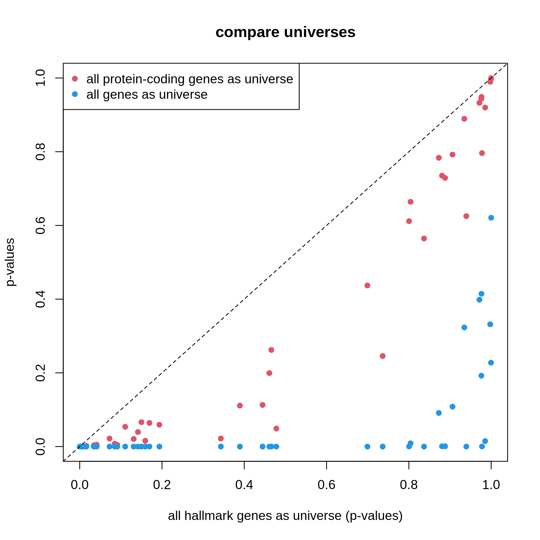
It is very straightforward to see, with a larger universe, there are more significant gene sets, which may produce potentially more false positives. This is definitely worse when using all genes in the genome as universe.
Based on the discussion in this section, the recommendation of using universe is:
- using protein-coding genes,
- using measured genes,
- or using a conservative way with clusterProfiler.
Visualization
clusterProfiler provides a rich set of visualization methods on the GSEA results, from simple visualization to complex ones. Complex visualizations are normally visually fancy but do not transfer too much useful information, and they should only be applied in very specific scenarios under very specific settings; while simple graphs normally do better jobs. Recently the visualization code in clusterProfiler has been moved to a new package enrichplot. Let’s first load the enrichplot package. The full sets of visualizations that enrichplot supports can be found from https://yulab-smu.top/biomedical-knowledge-mining-book/enrichplot.html.
We first re-generate the enrichment table.
R
library(enrichplot)
resTimeGO = enrichGO(gene = timeDEgenes,
keyType = "SYMBOL",
ont = "BP",
OrgDb = org.Mm.eg.db,
pvalueCutoff = 1,
qvalueCutoff = 1)
resTimeGOTable = as.data.frame(resTimeGO)
head(resTimeGOTable)
OUTPUT
ID Description GeneRatio BgRatio RichFactor
GO:0050900 GO:0050900 leukocyte migration 50/965 408/28832 0.1225490
GO:0006935 GO:0006935 chemotaxis 54/965 475/28832 0.1136842
GO:0042330 GO:0042330 taxis 54/965 477/28832 0.1132075
GO:0030595 GO:0030595 leukocyte chemotaxis 35/965 242/28832 0.1446281
GO:0060326 GO:0060326 cell chemotaxis 41/965 337/28832 0.1216617
GO:0071674 GO:0071674 mononuclear cell migration 32/965 229/28832 0.1397380
FoldEnrichment zScore pvalue p.adjust qvalue
GO:0050900 3.661485 10.075346 2.751321e-15 1.053782e-11 7.745382e-12
GO:0006935 3.396625 9.800882 5.186751e-15 1.053782e-11 7.745382e-12
GO:0042330 3.382383 9.763475 6.190224e-15 1.053782e-11 7.745382e-12
GO:0030595 4.321158 9.654694 3.373742e-13 4.307425e-10 3.165991e-10
GO:0060326 3.634975 9.054313 1.137629e-12 1.161974e-09 8.540597e-10
GO:0071674 4.175053 8.976588 8.861995e-12 6.891923e-09 5.065617e-09
geneID
GO:0050900 Tnfsf18/Sell/Slamf9/Fut7/Itga4/Mdk/Grem1/Ada/Prex1/Edn3/P2ry12/Il12a/S100a8/S100a9/Nbl1/Padi2/Bst1/Cxcl5/Ppbp/Pf4/Cxcl1/Ptn/Alox5/Trpm4/Hsd3b7/Itgam/Adam8/Ascl2/Gdf15/Calr/Enpp1/Aire/Ccl2/Ccl7/Ccl5/Ccr7/Aoc3/Itgb3/Ccl28/Lgals3/Ptk2b/Emp2/Apod/Retnlg/Plg/Fpr2/Dusp1/Ager/Il33/Ch25h
GO:0006935 Tnfsf18/Sell/Slamf9/Mdk/Grem1/Prex1/Edn3/P2ry12/Il12a/S100a7a/S100a8/S100a9/Lpar1/Ptgr1/Nbl1/Padi2/Bst1/Cxcl5/Ppbp/Pf4/Cxcl1/Ptn/Alox5/Ntf3/Trpm4/Hsd3b7/Itgam/Adam8/Lsp1/Calr/Ccl17/Robo3/Cmtm7/Ccl2/Ccl7/Ccl5/Ccl6/Ccr7/Itgb3/Tubb2b/Ccl28/Lgals3/Cmtm5/Ptk2b/Nr4a1/Casr/Retnlg/Fpr2/Dusp1/Ager/Stx3/Ch25h/Plxnb3/Nox1
GO:0042330 Tnfsf18/Sell/Slamf9/Mdk/Grem1/Prex1/Edn3/P2ry12/Il12a/S100a7a/S100a8/S100a9/Lpar1/Ptgr1/Nbl1/Padi2/Bst1/Cxcl5/Ppbp/Pf4/Cxcl1/Ptn/Alox5/Ntf3/Trpm4/Hsd3b7/Itgam/Adam8/Lsp1/Calr/Ccl17/Robo3/Cmtm7/Ccl2/Ccl7/Ccl5/Ccl6/Ccr7/Itgb3/Tubb2b/Ccl28/Lgals3/Cmtm5/Ptk2b/Nr4a1/Casr/Retnlg/Fpr2/Dusp1/Ager/Stx3/Ch25h/Plxnb3/Nox1
GO:0030595 Tnfsf18/Sell/Slamf9/Mdk/Grem1/Prex1/Edn3/Il12a/S100a8/S100a9/Nbl1/Padi2/Bst1/Cxcl5/Ppbp/Pf4/Cxcl1/Ptn/Alox5/Trpm4/Hsd3b7/Itgam/Adam8/Calr/Ccl2/Ccl7/Ccl5/Ccr7/Ccl28/Lgals3/Ptk2b/Retnlg/Fpr2/Dusp1/Ch25h
GO:0060326 Tnfsf18/Sell/Slamf9/Mdk/Grem1/Prex1/Edn3/Il12a/S100a8/S100a9/Lpar1/Nbl1/Padi2/Bst1/Cxcl5/Ppbp/Pf4/Cxcl1/Ptn/Alox5/Trpm4/Hsd3b7/Itgam/Adam8/Calr/Ccl17/Ccl2/Ccl7/Ccl5/Ccl6/Ccr7/Ccl28/Lgals3/Ptk2b/Nr4a1/Retnlg/Fpr2/Dusp1/Ch25h/Plxnb3/Nox1
GO:0071674 Tnfsf18/Slamf9/Fut7/Itga4/Mdk/Grem1/P2ry12/Il12a/Nbl1/Padi2/Alox5/Trpm4/Hsd3b7/Adam8/Ascl2/Calr/Enpp1/Aire/Ccl2/Ccl7/Ccl5/Ccr7/Itgb3/Lgals3/Ptk2b/Apod/Retnlg/Plg/Fpr2/Dusp1/Ager/Ch25h
Count
GO:0050900 50
GO:0006935 54
GO:0042330 54
GO:0030595 35
GO:0060326 41
GO:0071674 32barplot() and dotplot() generate plots for
a small number of significant gene sets. Note the two functions are
directly applied on resTimeGO returned by
enrichGO().
R
barplot(resTimeGO, showCategory = 20)
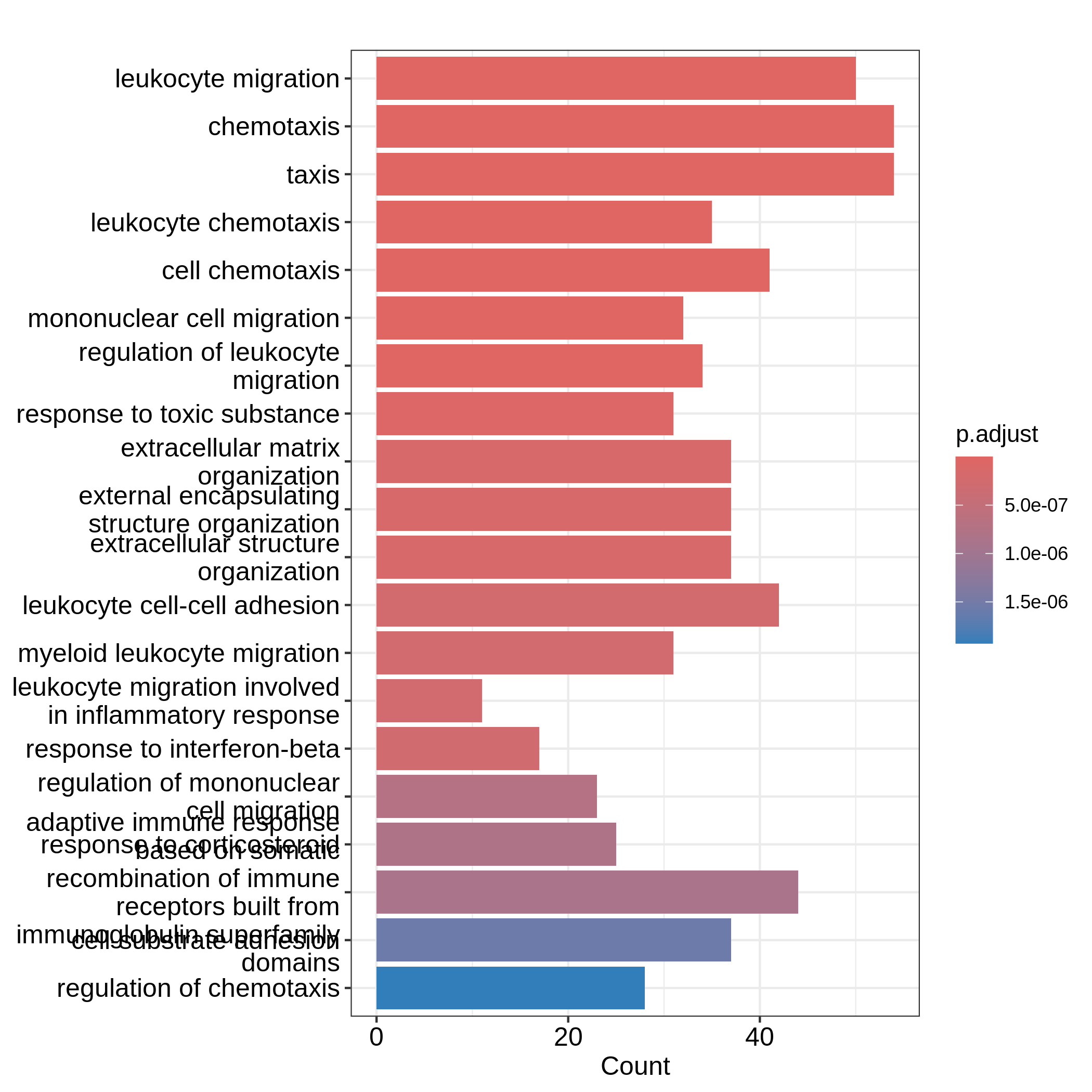
R
dotplot(resTimeGO, showCategory = 20)
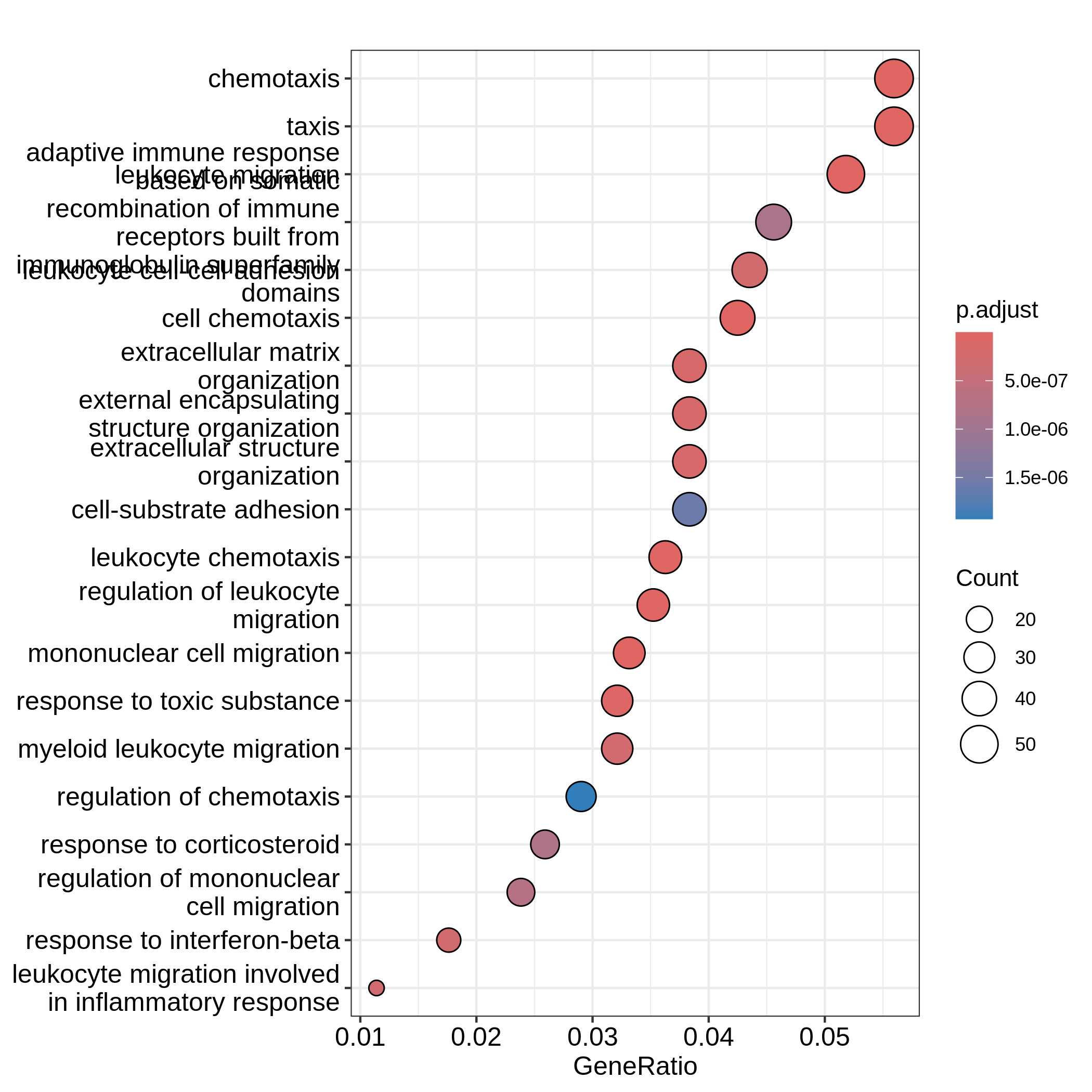
Barplots can map two variables to the plot, one to the height of bars
and the other to the colors of bars; while for dotplot, sizes of dots
can be mapped to a third variable. The variable names are in the colum
names of the result table. Both plots include the top 20 most
significant terms. On dotplot, terms are ordered by the values on x-axis
(the GeneRatio).
Now we need to talk about “what is a good visualization?”. The
essential two questions are “what is the key message a plot
transfers to readers?” and “what is the major graphical element
in the plot?”. In the barplot or dotplot, the major graphical
element which readers may notice the easiest is the height of bars or
the offset of dots to the origin. The most important message of the ORA
analysis is of course “the enrichment”. The two examples from
barplot() and dotplot() actually fail to
transfer such information to readers. In the first barplot where
"Count" is used as values on x-axis, the numer of DE genes
in gene sets is not a good measure of the enrichment because it has a
positive relation to the size of gene sets. A high value of
"Count" does not mean the gene set is more enriched.
It is the same reason for dotplot where "GeneRatio" is
used as values on x-axis. Gene ratio is calculated as the fraction of DE
genes from a certain gene set (GeneRatio = Count/Total_DE_Genes). The
dotplot puts multiple gene sets in the same plot and the aim is to
compare between gene sets, thus gene sets should be “scaled” to make
them comparable. "GeneRatio" is not scaled for different
gene sets and it still has a positive relation to the gene set size,
which can be observed in the dotplot where higher the gene ratio, larger
the dot size. Actually “GeneRatio” has the same effect as “Count”
(GeneRatio = Count/Total_DE_Genes), so as has been explained in the
previous paragraph, "GeneRatio" is not a good measure for
enrichment either.
Now let’s try to make a more reasonable barplot and dotplot to show the enrichment of ORA.
First, let’s define some metrics which measure the “enrichment” of DE genes on gene sets. Recall the denotations in the 2x2 contingency table (we are too far from that!). Let’s take these numbers from the enrichment table.
R
n_11 = resTimeGOTable$Count
n_10 = 983 # length(intersect(resTimeGO@gene, resTimeGO@universe))
n_01 = as.numeric(gsub("/.*$", "", resTimeGOTable$BgRatio))
n = 28943 # length(resTimeGO@universe)
Instead of using GeneRatio, we use the fraction of DE
genes in the gene sets which are kind of like a “scaled” value for all
gene sets. Let’s calculate it:
R
resTimeGOTable$DE_Ratio = n_11/n_01
resTimeGOTable$GS_size = n_01 # size of gene sets
Then intuitively, if a gene set has a higher DE_Ratio
value, we could say DE genes have a higher enrichment6 in it.
We can measure the enrichment in two other ways. First, the log2 fold enrichment, defined as:
\[\log_2(\mathrm{Fold\_enrichment}) = \frac{n_{11}/n_{10}}{n_{01}/n} = \frac{n_{11}/n_{01}}{n_{10}/n} = \frac{n_{11}n}{n_{10}n_{01}}\]
which is the log2 of the ratio of DE% in the gene set and DE% in the universe or the log2 of the ratio of gene_set% in the DE genes and gene_set% in the universe. The two are identical.
R
resTimeGOTable$log2_Enrichment = log( (n_11/n_10)/(n_01/n) )
Second, it is also common to use z-score which is
\[z = \frac{n_{11} - \mu}{\sigma}\]
where \(\mu\) and \(\sigma\) are the mean and standard deviation of the hypergeometric distribution. They can be calculated as:
R
hyper_mean = n_01*n_10/n
n_02 = n - n_01
n_20 = n - n_10
hyper_var = n_01*n_10/n * n_20*n_02/n/(n-1)
resTimeGOTable$zScore = (n_11 - hyper_mean)/sqrt(hyper_var)
We will use log2 fold change as the primary variable to map to bar
heights and DE_Ratio as the secondary variable to map to
colors. This can be done directly with the ggplot2
package. We also add the adjusted p-values as labels on the
bars.
In resTimeGOTable, gene sets are already ordered by the
significance, so we take the first 10 gene sets which are the 10 most
significant gene sets.
R
library(ggplot2)
ggplot(resTimeGOTable[1:10, ],
aes(x = log2_Enrichment, y = factor(Description, levels = rev(Description)),
fill = DE_Ratio)) +
geom_bar(stat = "identity") +
geom_text(aes(x = log2_Enrichment,
label = sprintf("%.2e", p.adjust)), hjust = 1, col = "white") +
ylab("")
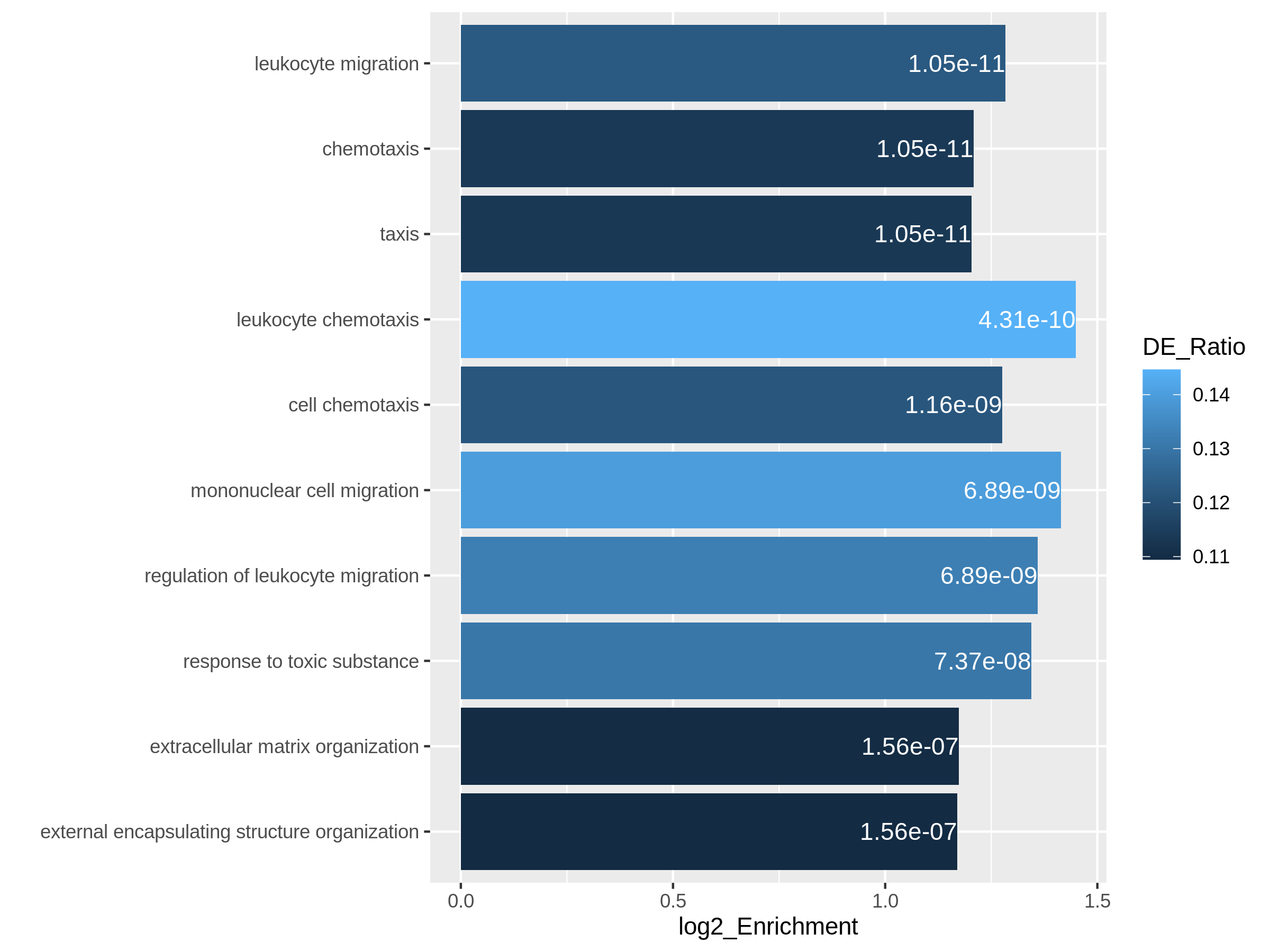
In the next example, we use z-score as the primary variable
to map to the offset to origin, DE_Ratio and
Count to map to dot colors and sizes.
R
ggplot(resTimeGOTable[1:10, ],
aes(x = zScore, y = factor(Description, levels = rev(Description)),
col = DE_Ratio, size = Count)) +
geom_point() +
ylab("")
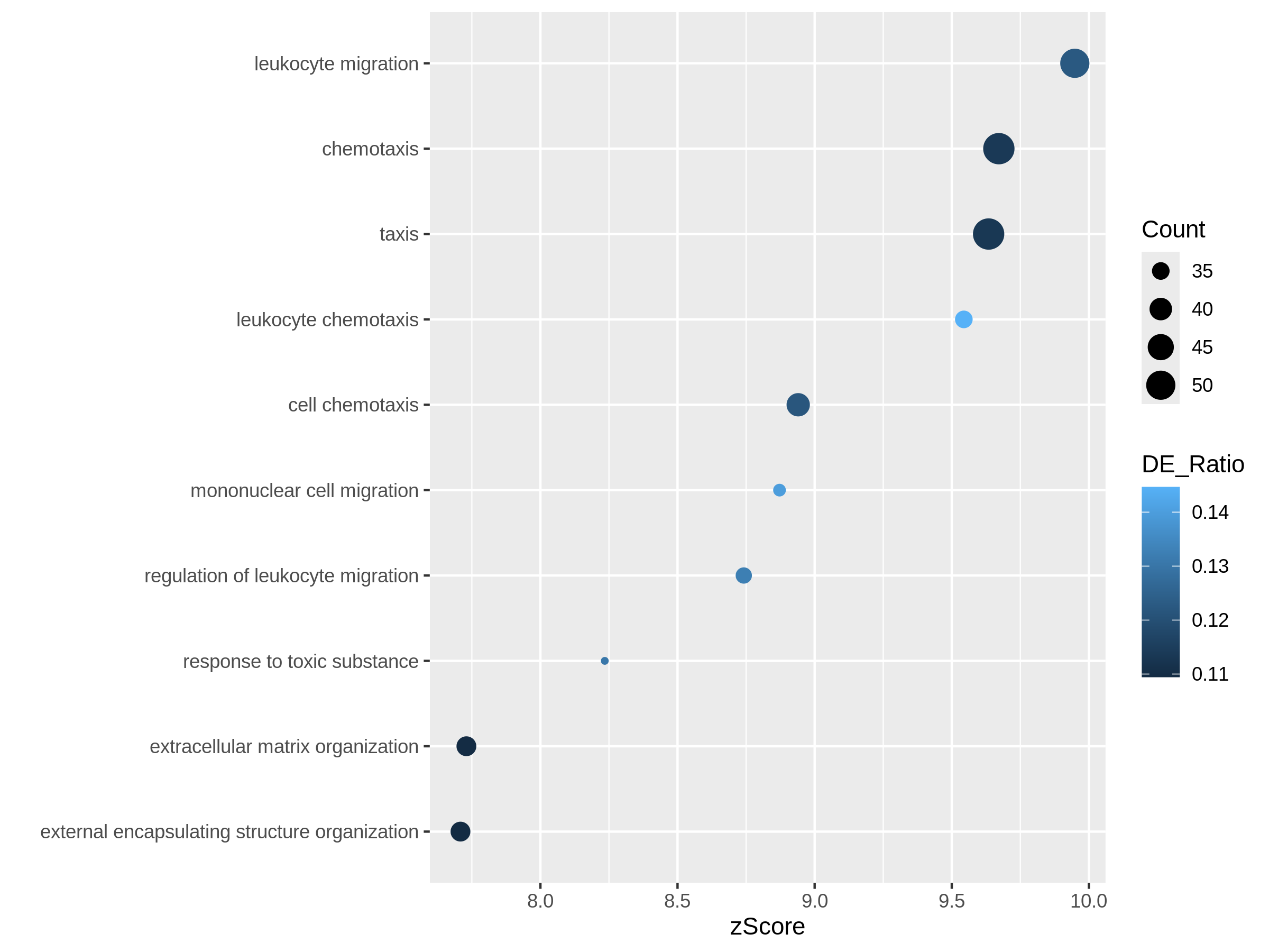
Both plots can highlight the gene set “leukocyte migration involved in inflammatory response” is relatively small but highly enriched.
Another useful visualization is the volcano plot. You may be aware of in differential expression analysis, in the volcano plot, x-axis corresponds to log2 fold changes of the differential expression, and y-axis corresponds to the adjusted p-values. It is actually similar here where we use log2 fold enrichment on x-axis.
Since we only look at the over-representation, the volcano plot is one-sided. We can set two cutoffs on the log2 fold enrichment and adjusted p-values, then the gene sets on the top right region can be thought as being both statistically significant and also biologically sensible.
R
ggplot(resTimeGOTable,
aes(x = log2_Enrichment, y = -log10(p.adjust),
color = DE_Ratio, size = GS_size)) +
geom_point() +
geom_hline(yintercept = -log10(0.01), lty = 2, col = "#444444") +
geom_vline(xintercept = 1.5, lty = 2, col = "#444444")
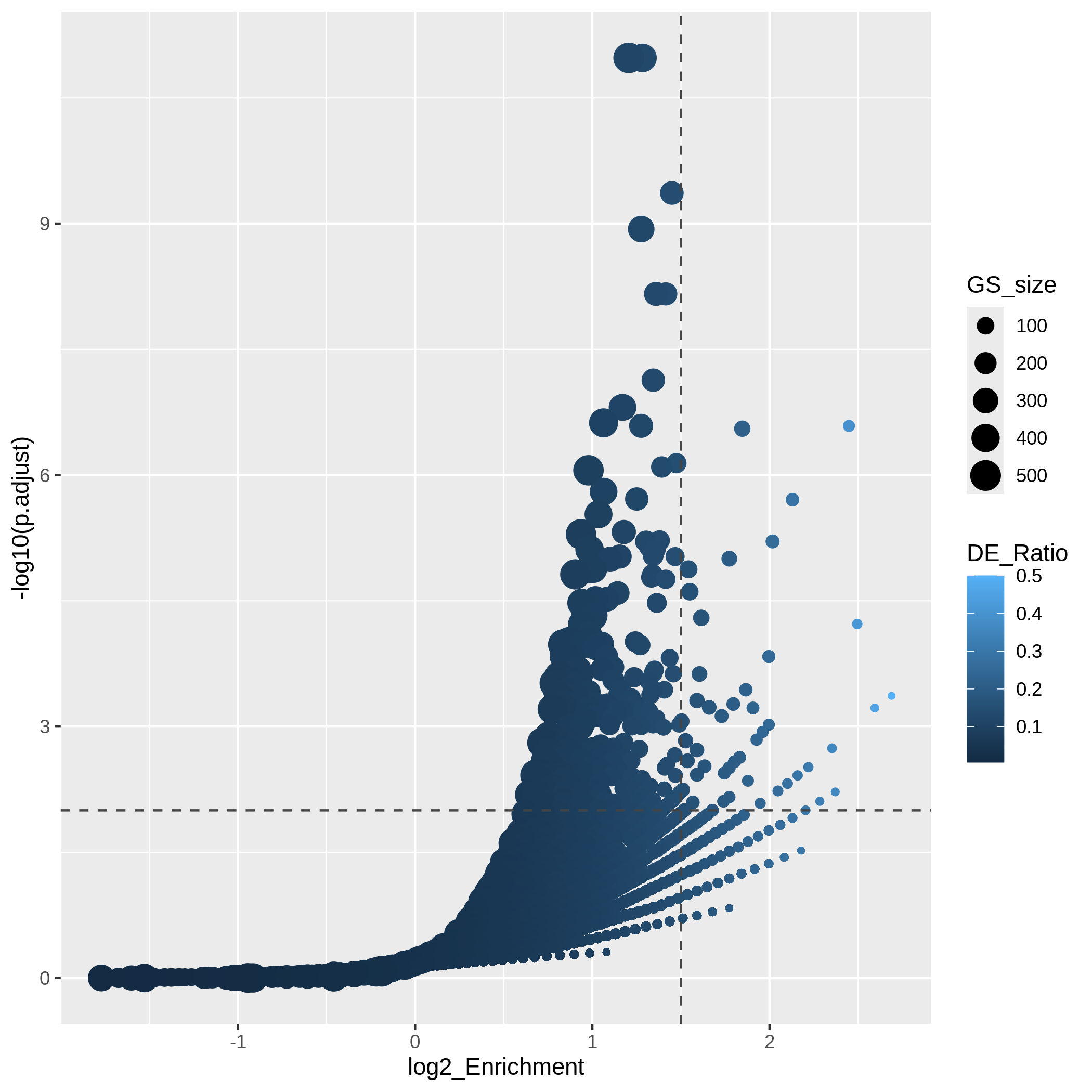
In the “volcano plot”, we can observe the plot is composed by a list
of curves. The trends are especially clear in the right bottom of the
plot. Actually each “curve” corresponds to a same "Count"
value (number of DE genes in a gene set). The volcano plot shows very
clearly that the enrichment has a positive relation to the gene set size
where a large gene set can easily reach a small p-value with a
small DE_ratio and a small log2 fold enrichment, while a small gene set
needs to have a large DE ratio to be significant.
It is also common that we perform ORA analysis on up-regulated genes and down-regulated separately. And we want to combine the significant gene sets from the two ORA analysis in one plot. In the following code, we first generate two enrichment tables for up-regulated genes and down-regulated separately.
R
# up-regulated genes
timeDEup <- as.data.frame(subset(resTime, padj < 0.05 & log2FoldChange > log2(1.5)))
timeDEupGenes <- rownames(timeDEup)
resTimeGOup = enrichGO(gene = timeDEupGenes,
keyType = "SYMBOL",
ont = "BP",
OrgDb = org.Mm.eg.db,
universe = rownames(se),
pvalueCutoff = 1,
qvalueCutoff = 1)
resTimeGOupTable = as.data.frame(resTimeGOup)
n_11 = resTimeGOupTable$Count
n_10 = length(intersect(resTimeGOup@gene, resTimeGOup@universe))
n_01 = as.numeric(gsub("/.*$", "", resTimeGOupTable$BgRatio))
n = length(resTimeGOup@universe)
resTimeGOupTable$log2_Enrichment = log( (n_11/n_10)/(n_01/n) )
# down-regulated genes
timeDEdown <- as.data.frame(subset(resTime, padj < 0.05 & log2FoldChange < -log2(1.5)))
timeDEdownGenes <- rownames(timeDEdown)
resTimeGOdown = enrichGO(gene = timeDEdownGenes,
keyType = "SYMBOL",
ont = "BP",
OrgDb = org.Mm.eg.db,
universe = rownames(se),
pvalueCutoff = 1,
qvalueCutoff = 1)
resTimeGOdownTable = as.data.frame(resTimeGOdown)
n_11 = resTimeGOdownTable$Count
n_10 = length(intersect(resTimeGOdown@gene, resTimeGOdown@universe))
n_01 = as.numeric(gsub("/.*$", "", resTimeGOdownTable$BgRatio))
n = length(resTimeGOdown@universe)
resTimeGOdownTable$log2_Enrichment = log( (n_11/n_10)/(n_01/n) )
As an example, let’s simply take the first 5 most significant terms for up-regulated genes and the first 5 most significant terms for down-regulated genes. The following ggplot2 code should be easy to read.
R
# The name of the 3rd term is too long, we wrap it into two lines.
resTimeGOupTable[3, "Description"] = paste(strwrap(resTimeGOupTable[3, "Description"]), collapse = "\n")
direction = c(rep("up", 5), rep("down", 5))
ggplot(rbind(resTimeGOupTable[1:5, ],
resTimeGOdownTable[1:5, ]),
aes(x = log2_Enrichment, y = factor(Description, levels = rev(Description)),
fill = direction)) +
geom_bar(stat = "identity") +
scale_fill_manual(values = c("up" = "red", "down" = "darkgreen")) +
geom_text(aes(x = log2_Enrichment,
label = sprintf("%.2e", p.adjust)), hjust = 1, col = "white") +
ylab("")
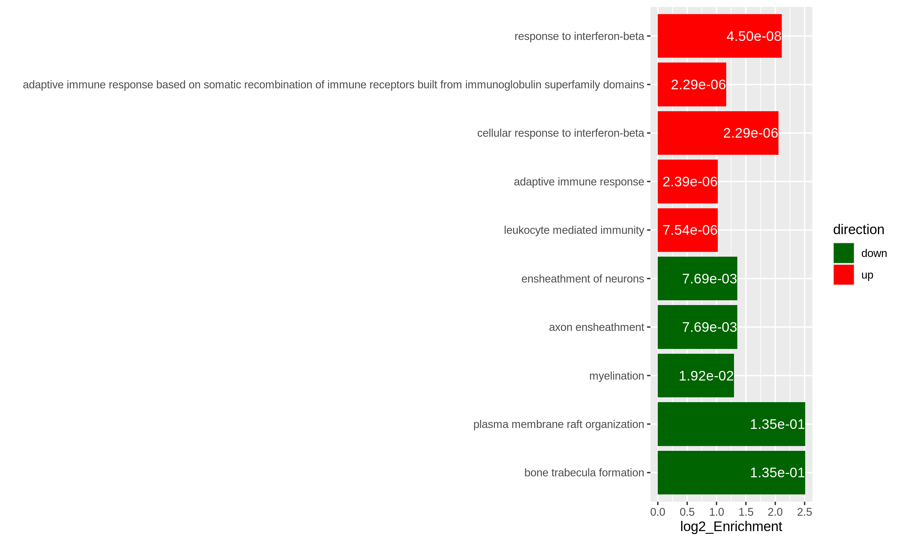
Specifically for GO enrichment, it is often that GO enrichment returns a long list of significant GO terms (e.g. several hundreds). This makes it difficult to summarize the common functions from the long list. The last package we will introduce is the simplifyEnrichment package which partitions GO terms into clusters based on their semantic similarity7 and summarizes their common functions via word clouds.
The input of the simplifyGO() function is a vector of GO
IDs. It is recommended to have at least 100 GO IDs for summarization and
visualization.
R
GO_ID = resTimeGOTable$ID[resTimeGOTable$p.adjust < 0.1]
library(simplifyEnrichment)
simplifyGO(GO_ID)
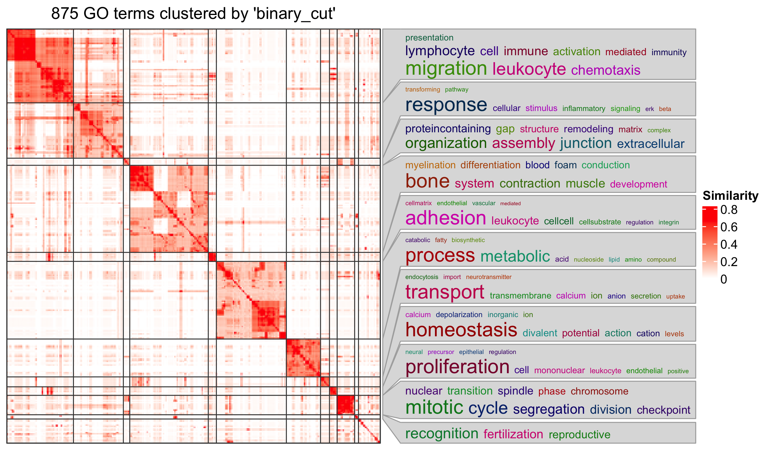
Further reading
ORA analysis actually applies a binary conversion on genes where genes pass the cutoff are set as 1 (DE gene) and others are set as 0 (non-DE gene). This binary transformation over-simplifies the problem and a lot of information are lost. There is second class of gene set enrichment analysis methods which takes the continuous gene-level score as input and weights the importance of a gene in the gene set. Please refer to Subramanian et. al. Gene set enrichment analysis: A knowledge-based approach for interpreting genome-wide expression profiles, PNAS 2005 for more information.
- ORA analysis is based on the gene counts and it is based on Fisher’s exact test or the hypergeometric distribution.
- In R, it is easy to obtain gene sets from a large number of sources.
Genes must be unique in each vector.↩︎
Also note
phyper()can be vectorized.↩︎The definition is from Wikipedia: https://en.wikipedia.org/wiki/Biological_pathway.↩︎
This is actually not true. Indeed
as.data.frame(resTimeGO)only returns the significant GO terms, but the complete enrichment table is still stored inresTimeGO@result. However, directly retrieving the slot of an S4 object is highly unrecommended.↩︎You can also use
select()function:select(org.Mm.eg.db, keys = timeDEgenes, keytype = "SYMBOL", column = "ENTREZID")↩︎If here the term “enrichment” does mean statistically.↩︎
The semantic similarity between GO terms considers the topological relations in the GO hierarchy.↩︎
Content from Next steps
Last updated on 2025-11-11 | Edit this page
Estimated time 20 minutes
Overview
Questions
- How to go further from here?
- What other types of analyses can be done with RNA-seq data?
Objectives
- Get an overview of usages of RNA-seq data that are not covered in this workshop.
Transcript-level analyses
The analyses covered in this workshop all assumed that we have generated a matrix with read counts for each gene. Some questions, however, require expression estimates on a more fine-grained level, typically individual transcript isoforms. This is the case, for example, if we would like to look for differences in expression of individual isoforms, or changes in splicing patterns induced by a specific treatment. As already mentioned in episode 1, some quantification tools (such as Salmon, kallisto and RSEM) do in fact estimate abundances on the transcript level. To perform transcript-level differential expression analysis, these estimates would be used directly, without aggregating them on the gene level. Some caution is warranted, however, as expression estimates for individual transcripts are often more noisy than after aggregation to the gene level. This is due to the high similarity often observed between different isoforms of a gene, which leads to higher uncertainty when mapping reads to transcripts. For this reason, several approaches have been developed specifically for performing differential expression analysis on the transcript level [@Zhu2019-swish, @Baldoni2023-catchsalmon].
Analysis of differential splicing, or differential transcript usage, differs from the differential expression analyses mentioned so far as it is concerned with changes in the relative abundances of the transcripts of a gene. Hence, considering the transcripts in isolation is no longer sufficient. A good resource for learning more about differential transcript usage with Bioconductor is provided by @Love2018-swimming.
De novo transcript assembly
In this lesson, we have assumed that we are working with a well-annotated transcriptome, that is, that we know the sequence of all expressed isoforms and how they are grouped together into genes. Depending on the organism or disease type we are interested in, this may or may not be a reasonable assumption. In situations where we do not believe that the annotated transcriptome is complete enough, we can use the RNA-seq data to assemble transcripts and create a custom annotation. This assembly can be performed either guided by a genome sequence (if one is available), or completely de novo. It should be noted that transcript assembly is a challenging task, which requires a deeply sequenced library to get the best results. In addition, data from more recent long-read sequencing technologies can be very helpful, as they are in principle able to sequence entire transcript molecules, thus circumventing the need for assembly. Methods for transcript assembly represent an active area of research. Recent review are provided e.g. by @Raghavan2022-denovo and @Amarasinghe2020-longread.
- RNA-seq data is very versatile and can be used for a number of different purposes. It is important, however, to carefully plan one’s analyses, to make sure that enough data is available and that abundances for appropriate features (e.g., genes, transcripts, or exons) are quantified.